
Comparing data.table reshape to duckdb and polars
Want to share your content on R-bloggers? click here if you have a blog, or here if you don't.
One element of the NSF POSE grant for data.table is to create benchmarks which can inform users about when data.table could be more performant than similar software. Two examples of similar software are duckdb and polars, which each provide in-memory database operations. This post explores the differences in computational requirements, and in functionality, for data reshaping operations.
Terminology and functions in R, data.table, and SQL
Data reshaping means changing the shape of the data, in order to get it into a more appropriate format, for learning/plotting/etc. In R we use the terms “wide” (many columns, few rows) and “long” (few columns, many rows) to describe the different data shapes (and these terms come from ?stats::reshape), whereas in SQL we use the terms “pivoted” and “unpivoted” to describe these two table types.
| R table type | SQL table type | rows | columns |
|---|---|---|---|
| long | unpivoted | many | few |
| wide | pivoted | few | many |
For the wide-to-long reshape operation, data.table has melt() and SQL has UNPIVOT; for the long-to-wide reshape operation, data.table has dcast() and SQL has PIVOT.
| Reshape operation | data.table function |
SQL function |
|---|---|---|
| Wide-to-long | melt |
UNPIVOT |
| Long-to-wide | dcast |
PIVOT |
Wide-to-long operations
We begin with a discussion of wide-to-long reshape operations, also known as unpivot in SQL.
Wide-to-long data reshape (unpivot) using data.table::melt
Wide-to-long reshape is often necessary before plotting. It is perhaps best explained using a simple example. Here we consider the iris data, which has four numeric columns:
library(data.table)
(iris.wide <- data.table(iris))
     Sepal.Length Sepal.Width Petal.Length Petal.Width   Species
            <num>       <num>        <num>       <num>    <fctr>
  1:          5.1         3.5          1.4         0.2    setosa
  2:          4.9         3.0          1.4         0.2    setosa
  3:          4.7         3.2          1.3         0.2    setosa
  4:          4.6         3.1          1.5         0.2    setosa
  5:          5.0         3.6          1.4         0.2    setosa
 ---
146:          6.7         3.0          5.2         2.3 virginica
147:          6.3         2.5          5.0         1.9 virginica
148:          6.5         3.0          5.2         2.0 virginica
149:          6.2         3.4          5.4         2.3 virginica
150:          5.9         3.0          5.1         1.8 virginica
What if we wanted to make a facetted histogram of the numeric iris data columns, with one panel/facet for each column? With ggplots we would use geom_histogram(aes(numeric_variable)), where numeric_variable would be the column name of a data table containing all of the numbers that we want to show in the histogram. To construct that table, we would have to first reshape to “long” (or unpivoted) format. To easily understand what the reshape operation does, we show a subset of the data (first and last rows) below:
(two.iris.wide <- iris.wide[c(1,.N)])
   Sepal.Length Sepal.Width Petal.Length Petal.Width   Species
          <num>       <num>        <num>       <num>    <fctr>
1:          5.1         3.5          1.4         0.2    setosa
2:          5.9         3.0          5.1         1.8 virginica
Note the table above has 8 numbers, arranged into a table of 2 rows and 4 columns. To reshape these data to “long” (or unpivoted) format, we can use data.table::melt, as in the code below.
melt(two.iris.wide, measure.vars=measure(part, dim, sep="."))
     Species   part    dim value
      <fctr> <char> <char> <num>
1:    setosa  Sepal Length   5.1
2: virginica  Sepal Length   5.9
3:    setosa  Sepal  Width   3.5
4: virginica  Sepal  Width   3.0
5:    setosa  Petal Length   1.4
6: virginica  Petal Length   5.1
7:    setosa  Petal  Width   0.2
8: virginica  Petal  Width   1.8
Note the table above has the same 8 numbers, but arranged into 1 column in a table with 8 rows, which is the desired input for ggplots. Also note that the reshaped column names (Petal.Length, Sepal.Width, etc) each consist of two components, which become two different columns in the output: part (Sepal or Petal) and dim (Length or Width). In the code above, we used sep="." to specify that we want to split all of the iris column names using a dot, and then reshape all of the columns whose names split into the max number of items. The corresponding column names of the output are specified as the arguments of measure(), and for more info about this functionality, please read its man page.
Below we do the same reshape with the full iris data set, this time using a regular expression (instead of the sep argument used above),
(iris.long <- melt(iris.wide, measure.vars=measure(part, dim, pattern="(.*)[.](.*)")))
       Species   part    dim value
        <fctr> <char> <char> <num>
  1:    setosa  Sepal Length   5.1
  2:    setosa  Sepal Length   4.9
  3:    setosa  Sepal Length   4.7
  4:    setosa  Sepal Length   4.6
  5:    setosa  Sepal Length   5.0
 ---
596: virginica  Petal  Width   2.3
597: virginica  Petal  Width   1.9
598: virginica  Petal  Width   2.0
599: virginica  Petal  Width   2.3
600: virginica  Petal  Width   1.8
In the code above, the pattern argument is a Perl-compatible regular expression, and columns that match the pattern will be reshaped. The pattern must contain the same number of capture groups (parentheses) as the number of other arguments to melt (part and dim), which are used for output column names. After reshaping, we plot the data in a histogram:
library(ggplot2)
ggplot()+
  geom_histogram(aes(
    value),
    bins=50,
    data=iris.long)+
  facet_grid(part ~ dim, labeller=label_both)
![]()
We can see in the plot above that there is a top strip for each dim and a right strip for each part, and each facet/panel contains a histogram of the corresponding subset of data.
Wide-to-long reshape via unpivot in polars
![]()
polars is an implementation of data frames in Rust, with bindings in R and Python. In polars, the wide-to-long data reshape operation is documented on the man page for unpivot, which explains that we must specify index and/or on (no support for separator, nor regex). In our case, we use the code below:
(iris.long.polars <- polars::as_polars_df(iris)$unpivot(
  index="Species",
  on=c("Sepal.Length","Petal.Length","Sepal.Width","Petal.Width"),
  variable_name="part.dim",
  value_name="cm"))
shape: (600, 3)
┌───────────┬──────────────┬─────┐
│ Species   ┆ part.dim     ┆ cm  │
│ ---       ┆ ---          ┆ --- │
│ cat       ┆ str          ┆ f64 │
╞═══════════╪══════════════╪═════╡
│ setosa    ┆ Sepal.Length ┆ 5.1 │
│ setosa    ┆ Sepal.Length ┆ 4.9 │
│ setosa    ┆ Sepal.Length ┆ 4.7 │
│ setosa    ┆ Sepal.Length ┆ 4.6 │
│ setosa    ┆ Sepal.Length ┆ 5.0 │
│ …         ┆ …            ┆ …   │
│ virginica ┆ Petal.Width  ┆ 2.3 │
│ virginica ┆ Petal.Width  ┆ 1.9 │
│ virginica ┆ Petal.Width  ┆ 2.0 │
│ virginica ┆ Petal.Width  ┆ 2.3 │
│ virginica ┆ Petal.Width  ┆ 1.8 │
└───────────┴──────────────┴─────┘
The output above is analogous to the result from data.table::melt, but with one column named part.dim instead of the two columns named part and dim, because polars does not support splitting the reshaped column names into more than one output column. So with polars, if we wanted separate part and dim columns, we would have to specify that in a separate step, after the reshape. Or we could just use facet_wrap instead of facet_grid, as in the code below:
ggplot()+
  geom_histogram(aes(
    cm),
    bins=50,
    data=iris.long.polars)+
  facet_wrap(. ~ part.dim, labeller=label_both)
![]()
We can see in the plot above that there is a facet for each of the variables, but only one part.dim strip for each, instead of two strips (part and dim), as was the case for the previous plot.
Wide-to-long reshape via UNPIVOT in duckdb
![]()
duckdb is a column-oriented database implemented in C++, with an R package that supports a DBI-compliant SQL interface. That means that we use R functions like DBI::dbGetQuery to get results, just like we would with any other database (Postgres, MySQL, etc). This is documented in the duckdb R API docs, which explain how to create a database connection, and then copy data from R to the database, as in the code below,
con <- DBI::dbConnect(duckdb::duckdb(), dbdir = ":memory:")
DBI::dbWriteTable(con, "iris_wide", iris)
The duckdb unpivot man page explains how to do wide-to-long reshape operations, which requires specifying names of columns to reshape (no support for separator, nor regex). In our case, we use the code below:
iris.long.duckdb <- DBI::dbGetQuery(con, '
UNPIVOT iris_wide
ON "Sepal.Length", "Petal.Length", "Sepal.Width", "Petal.Width"
INTO NAME part_dim
VALUE cm')
str(iris.long.duckdb)
'data.frame':   600 obs. of  3 variables:
 $ Species : Factor w/ 3 levels "setosa","versicolor",..: 1 1 1 1 1 1 1 1 1 1 ...
 $ part_dim: chr  "Sepal.Length" "Petal.Length" "Sepal.Width" "Petal.Width" ...
 $ cm      : num  5.1 1.4 3.5 0.2 4.9 1.4 3 0.2 4.7 1.3 ...
Above we use str to show a brief summary of the structure of the output, which is a data.frame with 600 rows. With duckdb, the output has one column named part_dim (dots in column names are not allowed so we use an underscore here instead), because it does not support splitting the reshaped column names into more than one output column. So with duckdb, if we wanted separate part and dim columns, we would have to specify that in a separate step, after the reshape.
Creating part and dim columns
Both polars and duckdb are not capable of producing the separate part and dim columns during the reshape operation, but we can always do it as a post-processing step. One way to do that, by specifying a separator, would be via data.table::tstrsplit, as in the code below:
data.table(iris.long.duckdb)[
, c("part","dim") := tstrsplit(part_dim, split="[.]")
][]
       Species     part_dim    cm   part    dim
        <fctr>       <char> <num> <char> <char>
  1:    setosa Sepal.Length   5.1  Sepal Length
  2:    setosa Petal.Length   1.4  Petal Length
  3:    setosa  Sepal.Width   3.5  Sepal  Width
  4:    setosa  Petal.Width   0.2  Petal  Width
  5:    setosa Sepal.Length   4.9  Sepal Length
 ---
596: virginica  Petal.Width   2.3  Petal  Width
597: virginica Sepal.Length   5.9  Sepal Length
598: virginica Petal.Length   5.1  Petal Length
599: virginica  Sepal.Width   3.0  Sepal  Width
600: virginica  Petal.Width   1.8  Petal  Width
The code above first converts to data.table, then uses the square brackets to assign new columns. Inside the square brackets, there is a walrus assignment:
,comma because there is no first argument (no subset, use all rows)c("part","dim")is the left side of the walrus:=assignment, which specifies the new column names to create.- on the right side of the walrus, the result of
tstrsplit(part_dim, split="[.]")is used as the value to assign to the new columns (part_dimis the column to split, and"[.]"is the regex to use for splitting). - Since
tstrsplitreturns a list of two character vectors, there will be two new columns.
Finally after the walrus square brackets, we use another empty square brackets [] to enable printing (there is no printing immediately after assigning new columns using the walrus operator).
Another way of doing that, by specifying a regex, would be via nc::capture_first_df (recently given the data.table Seal of Approval), as in the code below:
nc::capture_first_df(iris.long.duckdb, part_dim=list(
  part=".*",
  "[.]",
  dim=".*"))
       Species     part_dim    cm   part    dim
        <fctr>       <char> <num> <char> <char>
  1:    setosa Sepal.Length   5.1  Sepal Length
  2:    setosa Petal.Length   1.4  Petal Length
  3:    setosa  Sepal.Width   3.5  Sepal  Width
  4:    setosa  Petal.Width   0.2  Petal  Width
  5:    setosa Sepal.Length   4.9  Sepal Length
 ---
596: virginica  Petal.Width   2.3  Petal  Width
597: virginica Sepal.Length   5.9  Sepal Length
598: virginica Petal.Length   5.1  Petal Length
599: virginica  Sepal.Width   3.0  Sepal  Width
600: virginica  Petal.Width   1.8  Petal  Width
The code above specifies:
capture_first_df, a function for applying capturing regex to columns of a data frame;iris.long.duckdbis the input data frame, in which there is thepart_dimcolumn to split;part=".*", "[.]", dim=".*"makes the capturing regex; R argument names are used to define the new column names, based on the text captured in the corresponding regex (".*"means zero or more non-newline characters).
Both results above are data tables with extra cols part and dim. For visualization, these data tables could be used with either facet_grid or facet_wrap, similar to the examples above.
Reshape into multiple columns
Another kind of wide-to-long reshape involves reshaping into multiple columns. For example, in the iris data, we may wonder whether sepals are larger than petals (in terms of both length and width). To answer that question, we could make a scatterplot of y=Sepal versus x=Petal, with a facet/panel for each dimension (Length and Width). In the ggplot system, we would need to compute a data table with columns Sepal, Petal, and dim, and we can do that by specifying the value.name keyword to measure(), as in the code below:
(iris.long.parts <- melt(iris.wide, measure.vars=measure(value.name, dim, sep=".")))
       Species    dim Sepal Petal
        <fctr> <char> <num> <num>
  1:    setosa Length   5.1   1.4
  2:    setosa Length   4.9   1.4
  3:    setosa Length   4.7   1.3
  4:    setosa Length   4.6   1.5
  5:    setosa Length   5.0   1.4
 ---
296: virginica  Width   3.0   2.3
297: virginica  Width   2.5   1.9
298: virginica  Width   3.0   2.0
299: virginica  Width   3.4   2.3
300: virginica  Width   3.0   1.8
Again, the measure() function in the code above operates by splitting the input column names using sep, which results in two groups (Sepal.Width split into Sepal and Width, etc) for each of the measured columns. The value.name keyword indicates that each unique value in the first group (Sepal and Petal) should be used as the name of an output column. This functionality can be very convenient for some data reshaping tasks, but it is neither supported in polars, nor in duckdb. Going back to our original motivating problem, we can make the scatterplot using the code below,
ggplot()+
  theme_bw()+
  geom_abline(slope=1, intercept=0, color="grey")+
  geom_point(aes(
    Petal, Sepal),
    data=iris.long.parts)+
  facet_grid(. ~ dim, labeller=label_both)+
  coord_equal()
![]()
From the plot above, we see that all of the data points (black) are above the y=x line (grey), so we can conclude that sepals are indeed larger than petals, in terms of both length and width.
Wide-to-long performance comparison
We may also wonder which data reshaping functions work fastest for large data. To answer that question, we will use atime, which is an R package that allows us to see how much time/memory is required for computations in R, as a function of data size N. In the setup argument of the code below, we repeat the iris data for a certain number of rows N. The code in the other arguments is run for the time/memory measurement, and is very similar to the code presented in previous sections. One difference is that for data.table we use id.vars instead of measure(), to more closely match the arguments provided to the other unpivot functions (for a more fair comparison).
seconds.limit <- 0.1
unpivot.res <- atime::atime(
  N=2^seq(1,50),
  setup={
    (row.id.vec <- 1+(seq(0,N-1) %% nrow(iris)))
    N.df <- iris[row.id.vec,]
    N.dt <- data.table(N.df)
    polars_df <- polars::as_polars_df(N.df)
    duckdb::dbWriteTable(con, "iris_table", N.df, overwrite=TRUE)
  },
  seconds.limit=seconds.limit,
  "duckdb\nUNPIVOT"=DBI::dbGetQuery(con, 'UNPIVOT iris_table ON "Sepal.Length", "Petal.Length", "Sepal.Width", "Petal.Width" INTO NAME part_dim VALUE cm'),
  "polars\nunpivot"=polars_df$unpivot(index="Species", value_name="cm"),
  "data.table\nmelt"=melt(N.dt, id.vars="Species", value.name="cm"))
unpivot.refs <- atime::references_best(unpivot.res)
unpivot.pred <- predict(unpivot.refs)
plot(unpivot.pred)+coord_cartesian(xlim=c(1e1,1e7))
Loading required namespace: directlabels
Warning in ggplot2::scale_x_log10("N", breaks = meas[,
10^seq(ceiling(min(log10(N))), : log-10 transformation introduced infinite
values.
![]()
In the plot above, the computation time in seconds is plotted as a function of N, the number of input rows to reshape. The horizontal reference line is drawn at 0.1 seconds, and the N highlighted corresponds to the throughput given that time limit. When we compare the N values shown for the different methods, we see that data.table is comparable to polars (within 2x), and both are much faster than duckdb (about 10x).
Above there are several confounding factors in the comparison, most notably that data must be copied to duckdb and polars before and after processing. In contrast, data.table provides setDT and setDF functions, which can convert to/from data tables, without copying. So when data originates in R, or needs to come back to R, we should include the copy time for a more fair comparison. Below we run that comparison:
seconds.limit <- 0.1
unpivot.copy.res <- atime::atime(
  N=2^seq(1,50),
  setup={
    (row.id.vec <- 1+(seq(0,N-1) %% nrow(iris)))
    N.df <- iris[row.id.vec,]
  },
  seconds.limit=seconds.limit,
  "duckdb\ncopy+UNPIVOT"={
    duckdb::dbWriteTable(con, "iris_table", N.df, overwrite=TRUE)
    DBI::dbGetQuery(con, 'UNPIVOT iris_table ON "Sepal.Length", "Petal.Length", "Sepal.Width", "Petal.Width" INTO NAME part_dim VALUE cm')
  },
  "polars\ncopy+unpivot"={
    polars_df <- polars::as_polars_df(N.df)
    polars_unpivot <- polars_df$unpivot(index="Species", value_name="cm")
    as.data.frame(polars_unpivot)
  },
  "data.table\nset+melt"=setDF(melt(setDT(N.df), id.vars="Species", value.name="cm")))
unpivot.copy.refs <- atime::references_best(unpivot.copy.res)
unpivot.copy.pred <- predict(unpivot.copy.refs)
plot(unpivot.copy.pred)+coord_cartesian(xlim=c(1e1,1e7))
Warning in ggplot2::scale_x_log10("N", breaks = meas[,
10^seq(ceiling(min(log10(N))), : log-10 transformation introduced infinite
values.
![]()
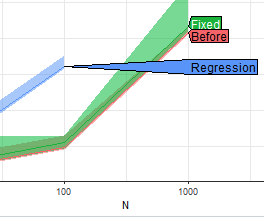
The result above shows that data.table is most efficient in terms of computation time. In this comparison, data.table is clearly faster than polars (about 10x), and much faster than duckdb (about 100x).
Wide-to-long summary of functionality
![]()
In this section, we showed that data.table provides an efficient and feature-rich implementation of wide-to-long data reshaping. * measure() allows specification of columns to reshape using either a separator or a regular expression pattern. In contrast, duckdb nor polars require specifying input column names (no support for separator, nor regex), and output column post-processing, which is less convenient. * The value.name keyword can be used to reshape into multiple output columns, which is required for some kinds of reshape operations (no way to do that in duckdb/polars). * setDT and setDF can be used to avoid un-necessary copies with data.table. In contrast, duckdb/polars require copies to/from regular R memory, which can add significant time/memory requirements. * data.table was fastest and most memory efficient in the comparisons we examined (both with and without consideration of copying).
The table below summarizes support for different features in each software package (dash - means no support).
| how to specify | data.table |
polars |
duckdb |
|---|---|---|---|
| function | melt |
unpivot |
UNPIVOT |
| reshape cols | measure.vars |
on |
ON |
| other cols | id.vars |
index |
- |
| output name (data) | value.name |
value_name |
VALUE |
| output name (columns) | variable.name |
variable_name |
INTO NAME |
| separator | sep |
- | - |
| regex | pattern |
- | - |
| multiple outputs | value.name |
- | - |
| avoid copies | setDT, setDF |
- | - |
Long-to-wide operations
Another kind of reshape operation starts with a long table (many rows, few cols), and creates a wide table (many cols, few rows). I frequently use this operation when comparing results of machine learning algorithms (computing mean/SD over folds, p-values, etc). For examples of those use cases, please read my blog about Visualizing prediction error.
Long-to-wide data reshape using data.table::dcast
Here we continue with the iris data example. We will present three different reshape operations involving the iris data. The code below adds a column flower which contains the row number.
iris.wide[, flower := .I][]
     Sepal.Length Sepal.Width Petal.Length Petal.Width   Species flower
            <num>       <num>        <num>       <num>    <fctr>  <int>
  1:          5.1         3.5          1.4         0.2    setosa      1
  2:          4.9         3.0          1.4         0.2    setosa      2
  3:          4.7         3.2          1.3         0.2    setosa      3
  4:          4.6         3.1          1.5         0.2    setosa      4
  5:          5.0         3.6          1.4         0.2    setosa      5
 ---
146:          6.7         3.0          5.2         2.3 virginica    146
147:          6.3         2.5          5.0         1.9 virginica    147
148:          6.5         3.0          5.2         2.0 virginica    148
149:          6.2         3.4          5.4         2.3 virginica    149
150:          5.9         3.0          5.1         1.8 virginica    150
Then we do a wide-to-long reshape using the code below (same as previous section),
(iris.long.i <- melt(iris.wide, measure.vars=measure(part, dim, sep=".")))
       Species flower   part    dim value
        <fctr>  <int> <char> <char> <num>
  1:    setosa      1  Sepal Length   5.1
  2:    setosa      2  Sepal Length   4.9
  3:    setosa      3  Sepal Length   4.7
  4:    setosa      4  Sepal Length   4.6
  5:    setosa      5  Sepal Length   5.0
 ---
596: virginica    146  Petal  Width   2.3
597: virginica    147  Petal  Width   1.9
598: virginica    148  Petal  Width   2.0
599: virginica    149  Petal  Width   2.3
600: virginica    150  Petal  Width   1.8
The table above has an additional column for flower, which we use in the code below on the left side of the formula (used to define output rows), along with part + dim on the right side of the formula (used to define output columns). The code below can therefore be used to reshape the data back into their original wide format:
dcast(# wide reshape 1
  data=iris.long.i,
  formula=flower + Species ~ part + dim,
  sep=".")
Key: <flower, Species>
     flower   Species Petal.Length Petal.Width Sepal.Length Sepal.Width
      <int>    <fctr>        <num>       <num>        <num>       <num>
  1:      1    setosa          1.4         0.2          5.1         3.5
  2:      2    setosa          1.4         0.2          4.9         3.0
  3:      3    setosa          1.3         0.2          4.7         3.2
  4:      4    setosa          1.5         0.2          4.6         3.1
  5:      5    setosa          1.4         0.2          5.0         3.6
 ---
146:    146 virginica          5.2         2.3          6.7         3.0
147:    147 virginica          5.0         1.9          6.3         2.5
148:    148 virginica          5.2         2.0          6.5         3.0
149:    149 virginica          5.4         2.3          6.2         3.4
150:    150 virginica          5.1         1.8          5.9         3.0
We can see that the result above is almost the same as the original iris data (but with the columns in a different order). Another kind of reshape involves computing an aggregation function, such as mean. Note in the code below that . on the right side of the formula indicates a single output column.
dcast(# wide reshape 2
  data=iris.long.i,
  formula=Species + part + dim ~ .,
  fun.aggregate=mean,
  sep=".")
Key: <Species, part, dim>
       Species   part    dim     .
        <fctr> <char> <char> <num>
 1:     setosa  Petal Length 1.462
 2:     setosa  Petal  Width 0.246
 3:     setosa  Sepal Length 5.006
 4:     setosa  Sepal  Width 3.428
 5: versicolor  Petal Length 4.260
 6: versicolor  Petal  Width 1.326
 7: versicolor  Sepal Length 5.936
 8: versicolor  Sepal  Width 2.770
 9:  virginica  Petal Length 5.552
10:  virginica  Petal  Width 2.026
11:  virginica  Sepal Length 6.588
12:  virginica  Sepal  Width 2.974
The output above has a row for every unique combination of Species, part, and dim, and a column (.)` for the mean of the corresponding data. The more complex reshape below involves multiple aggregations, and multiple value variables.
options(width=100)
dcast(# wide reshape 3
  data=iris.long.parts,
  formula=dim ~ Species,
  fun.aggregate=list(mean,sd),
  value.var=c("Sepal","Petal"))
Key: <dim>
      dim Sepal_mean_setosa Sepal_mean_versicolor Sepal_mean_virginica Petal_mean_setosa
   <char>             <num>                 <num>                <num>             <num>
1: Length             5.006                 5.936                6.588             1.462
2:  Width             3.428                 2.770                2.974             0.246
   Petal_mean_versicolor Petal_mean_virginica Sepal_sd_setosa Sepal_sd_versicolor
                   <num>                <num>           <num>               <num>
1:                 4.260                5.552       0.3524897           0.5161711
2:                 1.326                2.026       0.3790644           0.3137983
   Sepal_sd_virginica Petal_sd_setosa Petal_sd_versicolor Petal_sd_virginica
                <num>           <num>               <num>              <num>
1:          0.6358796       0.1736640           0.4699110          0.5518947
2:          0.3224966       0.1053856           0.1977527          0.2746501
The output above includes two rows, and a column for every unique combination of value.var (Sepal or Petal), of fun.aggregate (mean or sd), and of Species (setosa, versicolor, virginica).
Long-to-wide reshape in polars
polars supports long-to-wide reshape via the pivot method, as in the code below.
(polars.wide <- polars::as_polars_df(
  iris.long.i
)$pivot(# wide reshape 1
  on=c("part","dim"),
  index=c("flower","Species"),
  values="value"))
shape: (150, 6)
┌────────┬───────────┬───────────────────┬───────────────────┬──────────────────┬──────────────────┐
│ flower ┆ Species   ┆ {"Sepal","Length" ┆ {"Sepal","Width"} ┆ {"Petal","Length ┆ {"Petal","Width" │
│ ---    ┆ ---       ┆ }                 ┆ ---               ┆ "}               ┆ }                │
│ i32    ┆ cat       ┆ ---               ┆ f64               ┆ ---              ┆ ---              │
│        ┆           ┆ f64               ┆                   ┆ f64              ┆ f64              │
╞════════╪═══════════╪═══════════════════╪═══════════════════╪══════════════════╪══════════════════╡
│ 1      ┆ setosa    ┆ 5.1               ┆ 3.5               ┆ 1.4              ┆ 0.2              │
│ 2      ┆ setosa    ┆ 4.9               ┆ 3.0               ┆ 1.4              ┆ 0.2              │
│ 3      ┆ setosa    ┆ 4.7               ┆ 3.2               ┆ 1.3              ┆ 0.2              │
│ 4      ┆ setosa    ┆ 4.6               ┆ 3.1               ┆ 1.5              ┆ 0.2              │
│ 5      ┆ setosa    ┆ 5.0               ┆ 3.6               ┆ 1.4              ┆ 0.2              │
│ …      ┆ …         ┆ …                 ┆ …                 ┆ …                ┆ …                │
│ 146    ┆ virginica ┆ 6.7               ┆ 3.0               ┆ 5.2              ┆ 2.3              │
│ 147    ┆ virginica ┆ 6.3               ┆ 2.5               ┆ 5.0              ┆ 1.9              │
│ 148    ┆ virginica ┆ 6.5               ┆ 3.0               ┆ 5.2              ┆ 2.0              │
│ 149    ┆ virginica ┆ 6.2               ┆ 3.4               ┆ 5.4              ┆ 2.3              │
│ 150    ┆ virginica ┆ 5.9               ┆ 3.0               ┆ 5.1              ┆ 1.8              │
└────────┴───────────┴───────────────────┴───────────────────┴──────────────────┴──────────────────┘
names(polars.wide)
[1] "flower"                 "Species"                "{\"Sepal\",\"Length\"}"
[4] "{\"Sepal\",\"Width\"}"  "{\"Petal\",\"Length\"}" "{\"Petal\",\"Width\"}"
The output above is consistent with the results from data.table::dcast, and the original iris data, although the names are unusual (with curly braces and double quotes). The next reshape example below shows that we need to create a dummy variable to use as the on argument.
polars::as_polars_df(
  iris.long.i[, dummy := "."]
)$pivot(# wide reshape 2
  on="dummy", # have to create dummy var for on.
  index=c("Species","part","dim"),
  values="value",
  aggregate_function="mean")
shape: (12, 4)
┌────────────┬───────┬────────┬───────┐
│ Species    ┆ part  ┆ dim    ┆ .     │
│ ---        ┆ ---   ┆ ---    ┆ ---   │
│ cat        ┆ str   ┆ str    ┆ f64   │
╞════════════╪═══════╪════════╪═══════╡
│ setosa     ┆ Sepal ┆ Length ┆ 5.006 │
│ versicolor ┆ Sepal ┆ Length ┆ 5.936 │
│ virginica  ┆ Sepal ┆ Length ┆ 6.588 │
│ setosa     ┆ Sepal ┆ Width  ┆ 3.428 │
│ versicolor ┆ Sepal ┆ Width  ┆ 2.77  │
│ …          ┆ …     ┆ …      ┆ …     │
│ versicolor ┆ Petal ┆ Length ┆ 4.26  │
│ virginica  ┆ Petal ┆ Length ┆ 5.552 │
│ setosa     ┆ Petal ┆ Width  ┆ 0.246 │
│ versicolor ┆ Petal ┆ Width  ┆ 1.326 │
│ virginica  ┆ Petal ┆ Width  ┆ 2.026 │
└────────────┴───────┴────────┴───────┘
The output above is consistent with the results from data.table::dcast. Currently polars only supports a single aggregation function, so we can not calculate both mean and sd at the same time, but we can at least do the mean for multiple values in the code below:
polars::as_polars_df(
  iris.long.parts
)$pivot(# wide reshape 3
  on="Species",
  index="dim",
  values=c("Sepal","Petal"),
  aggregate_function="mean")#multiple agg not supported.
shape: (2, 7)
┌────────┬──────────────┬──────────────┬──────────────┬──────────────┬──────────────┬──────────────┐
│ dim    ┆ Sepal_setosa ┆ Sepal_versic ┆ Sepal_virgin ┆ Petal_setosa ┆ Petal_versic ┆ Petal_virgin │
│ ---    ┆ ---          ┆ olor         ┆ ica          ┆ ---          ┆ olor         ┆ ica          │
│ str    ┆ f64          ┆ ---          ┆ ---          ┆ f64          ┆ ---          ┆ ---          │
│        ┆              ┆ f64          ┆ f64          ┆              ┆ f64          ┆ f64          │
╞════════╪══════════════╪══════════════╪══════════════╪══════════════╪══════════════╪══════════════╡
│ Length ┆ 5.006        ┆ 5.936        ┆ 6.588        ┆ 1.462        ┆ 4.26         ┆ 5.552        │
│ Width  ┆ 3.428        ┆ 2.77         ┆ 2.974        ┆ 0.246        ┆ 1.326        ┆ 2.026        │
└────────┴──────────────┴──────────────┴──────────────┴──────────────┴──────────────┴──────────────┘
Above we see the result only has 6 columns (for mean), whereas the analogous result from data.table::dcast above had 12 columns (with additionally the sd).
Long-to-wide reshape in duckdb
duckdb supports long-to-wide reshape via the SQL PIVOT command, which can be used to recover the original iris data via the command below:
duckdb::dbWriteTable(con, "iris_long_i", iris.long.i, overwrite=TRUE)
iris.wide.again.duckdb <- DBI::dbGetQuery(# wide reshape 1
  con, '
PIVOT iris_long_i
ON part,dim
USING sum(value)
GROUP BY flower,Species
ORDER BY flower')
str(iris.wide.again.duckdb)
'data.frame':   150 obs. of  6 variables:
 $ flower      : int  1 2 3 4 5 6 7 8 9 10 ...
 $ Species     : Factor w/ 3 levels "setosa","versicolor",..: 1 1 1 1 1 1 1 1 1 1 ...
 $ Petal_Length: num  1.4 1.4 1.3 1.5 1.4 1.7 1.4 1.5 1.4 1.5 ...
 $ Petal_Width : num  0.2 0.2 0.2 0.2 0.2 0.4 0.3 0.2 0.2 0.1 ...
 $ Sepal_Length: num  5.1 4.9 4.7 4.6 5 5.4 4.6 5 4.4 4.9 ...
 $ Sepal_Width : num  3.5 3 3.2 3.1 3.6 3.9 3.4 3.4 2.9 3.1 ...
We can see that the result above is consistent with the previous sections. The code below uses mean as an aggregation function.
DBI::dbGetQuery(# wide reshape 2
  con, '
PIVOT iris_long_i
USING mean(value)
AS "."
GROUP BY Species,part,dim')
      Species  part    dim     .
1  versicolor Sepal Length 5.936
2   virginica Sepal Length 6.588
3  versicolor Sepal  Width 2.770
4   virginica Sepal  Width 2.974
5      setosa Petal Length 1.462
6      setosa Petal  Width 0.246
7      setosa Sepal Length 5.006
8      setosa Sepal  Width 3.428
9   virginica Petal Length 5.552
10  virginica Petal  Width 2.026
11 versicolor Petal Length 4.260
12 versicolor Petal  Width 1.326
The result above is consistent with previous results. Finally, we can do multiple aggregations via the code below, which requires enumerating each combination of aggregation function and input column to aggregate.
duckdb::dbWriteTable(con, "iris_long_parts", iris.long.parts, overwrite=TRUE)
DBI::dbGetQuery(# wide reshape 3
  con, '
PIVOT iris_long_parts
ON Species
USING
 mean(Sepal) AS Sepal_mean,
 stddev(Sepal) AS Sepal_sd,
 mean(Petal) AS Petal_mean,
 stddev(Petal) AS Petal_sd
GROUP BY dim')
     dim setosa_Sepal_mean setosa_Sepal_sd setosa_Petal_mean setosa_Petal_sd versicolor_Sepal_mean
1 Length             5.006       0.3524897             1.462       0.1736640                 5.936
2  Width             3.428       0.3790644             0.246       0.1053856                 2.770
  versicolor_Sepal_sd versicolor_Petal_mean versicolor_Petal_sd virginica_Sepal_mean
1           0.5161711                 4.260           0.4699110                6.588
2           0.3137983                 1.326           0.1977527                2.974
  virginica_Sepal_sd virginica_Petal_mean virginica_Petal_sd
1          0.6358796                5.552          0.5518947
2          0.3224966                2.026          0.2746501
The result above is consistent with the result from data.table::dcast. Because all combinations of aggregation/columns must be enumerated, the duckdb code is a bit more repetitive than the corresponding data.table code (which is more convenient).
Long-to-wide performance comparison
Below we conduct an atime benchmark to measure the computation time of the reshape operation (without controlling for the copy operation).
seconds.limit <- 0.1
pivot.res <- atime::atime(
  N=2^seq(1,50),
  setup={
    (row.id.vec <- 1+(seq(0,N-1) %% nrow(iris.long.i)))
    N.dt <- iris.long.i[row.id.vec]
    N.df <- data.frame(N.dt)
    N_polars <- polars::as_polars_df(N.df)
    duckdb::dbWriteTable(con, "iris_long_i", N.df, overwrite=TRUE)
  },
  seconds.limit=seconds.limit,
  "duckdb\nPIVOT"=DBI::dbGetQuery(con, 'PIVOT iris_long_i USING mean(value) AS "." GROUP BY Species,part,dim'),
  "polars\npivot"=N_polars$pivot(on="dummy", index=c("Species","part","dim"), values="value", aggregate_function="mean"),
  "data.table\ndcast"=dcast(N.dt, Species + part + dim ~ ., mean))
pivot.refs <- atime::references_best(pivot.res)
pivot.pred <- predict(pivot.refs)
plot(pivot.pred)+coord_cartesian(xlim=c(1e1,1e7))
Warning in ggplot2::scale_x_log10("N", breaks = meas[, 10^seq(ceiling(min(log10(N))), : log-10
transformation introduced infinite values.
![]()
The result above shows that data.table::dcast is about as fast as the others (bottom facet), although duckdb is slightly faster, and polars is slightly slower (less than 2x). Below we run a more complex benchmark which also measures computation time for the copy operation (in addition to the reshape).
seconds.limit <- 0.1
pivot.copy.res <- atime::atime(
  N=2^seq(1,50),
  setup={
    (row.id.vec <- 1+(seq(0,N-1) %% nrow(iris.long.i)))
    N.df <- data.frame(iris.long.i[row.id.vec])
  },
  seconds.limit=seconds.limit,
  "duckdb\ncopy+PIVOT"={
    duckdb::dbWriteTable(con, "iris_long_i", N.df, overwrite=TRUE)
    DBI::dbGetQuery(con, 'PIVOT iris_long_i USING mean(value) AS "." GROUP BY Species,part,dim')
  },
  "polars\ncopy+pivot"={
    polars_pivot <- polars::as_polars_df(
      N.df
    )$pivot(# wide reshape 2
      on="dummy", # have to create dummy var for on.
      index=c("Species","part","dim"),
      values="value",
      aggregate_function="mean")
    as.data.frame(polars_pivot)
  },
  "data.table\nset+dcast"=setDF(dcast(setDT(N.df), Species + part + dim ~ ., mean)))
pivot.copy.refs <- atime::references_best(pivot.copy.res)
pivot.copy.pred <- predict(pivot.copy.refs)
plot(pivot.copy.pred)+coord_cartesian(xlim=c(1e1,1e7))
Warning in ggplot2::scale_x_log10("N", breaks = meas[, 10^seq(ceiling(min(log10(N))), : log-10
transformation introduced infinite values.
![]()
The result above shows that data.table is quite a bit faster than the others (5x or more).
Summary of long-to-wide reshaping
In this section, we showed that data.table provides an efficient and feature-rich implementation of long-to-wide data reshaping. * The formula interface allows specifying a dot (.) which is a convenient way to specify output of only one row/column. In contrast, polars requires creating a dummy variable to do that. * The fun.aggregate argument may be a list of functions, each of which will be used on each of the value.var (a convenient way of specifying all combinations). In contrast, duckdb requires specifying each combination separately (more tedious/error-prone), and polars only supports one aggregation function (not a list).
| how to specify | data.table |
polars |
duckdb |
|---|---|---|---|
| function | dcast |
pivot |
PIVOT |
| rows | LHS of formula | index |
GROUP BY |
| columns | RHS of formula | on |
ON |
| no columns | dot . |
dummy variable | omit ON |
| values | value.var |
values |
USING |
| aggregation | aggregate.fun |
aggregate_function |
USING |
| multiple agg. | all combinations | one function | specified combinations |
Conclusion
We have compared the reshaping functions in data.table to duckdb and polars. Although all three provide similar functionality for basic operations, we observed that data.table has several advantages for advanced/complex/efficient operations (reshaping columns which match a regex/separator, reshaping into multiple columns, avoiding copies, multiple aggregation). We also observed that the speed of data.table functions is comparable, if not faster, than the other packages.
Attribution
Parts of this blog post were copied from my more extensive comparison blog.
Session info
sessionInfo()
R version 4.4.1 (2024-06-14)
Platform: aarch64-apple-darwin20
Running under: macOS Sonoma 14.7

Matrix products: default
BLAS:   /Library/Frameworks/R.framework/Versions/4.4-arm64/Resources/lib/libRblas.0.dylib
LAPACK: /Library/Frameworks/R.framework/Versions/4.4-arm64/Resources/lib/libRlapack.dylib;  LAPACK version 3.12.0

locale:
[1] en_US.UTF-8/en_US.UTF-8/en_US.UTF-8/C/en_US.UTF-8/en_US.UTF-8

time zone: America/Los_Angeles
tzcode source: internal

attached base packages:
[1] stats     graphics  grDevices utils     datasets  methods   base

other attached packages:
[1] ggplot2_3.5.1     data.table_1.15.4

loaded via a namespace (and not attached):
 [1] gtable_0.3.5           jsonlite_1.8.8         dplyr_1.1.4            compiler_4.4.1
 [5] tidyselect_1.2.1       directlabels_2024.1.21 scales_1.3.0           yaml_2.3.8
 [9] fastmap_1.1.1          lattice_0.22-6         R6_2.5.1               labeling_0.4.3
[13] generics_0.1.3         knitr_1.48             htmlwidgets_1.6.4      tibble_3.2.1
[17] polars_0.20.0          munsell_0.5.1          atime_2024.4.23        DBI_1.2.2
[21] pillar_1.9.0           rlang_1.1.3            utf8_1.2.4             xfun_0.46
[25] quadprog_1.5-8         cli_3.6.2              withr_3.0.0            magrittr_2.0.3
[29] digest_0.6.35          grid_4.4.1             rstudioapi_0.16.0      nc_2024.2.21
[33] lifecycle_1.0.4        vctrs_0.6.5            bench_1.1.3            evaluate_0.23
[37] glue_1.7.0             farver_2.1.1           duckdb_1.1.1           profmem_0.6.0
[41] fansi_1.0.6            colorspace_2.1-0       rmarkdown_2.27         tools_4.4.1
[45] pkgconfig_2.0.3        htmltools_0.5.8.1


R-bloggers.com offers daily e-mail updates about R news and tutorials about learning R and many other topics. Click here if you're looking to post or find an R/data-science job.
Want to share your content on R-bloggers? click here if you have a blog, or here if you don't.