The R {targets} package is a pipeline tool for statistics, data science, and machine learning in R. The package allows you to write and maintain reproducible R workflows in pipelines that run only when necessary (e.g., either data or code has changed). The best part is – you’ll learn ...

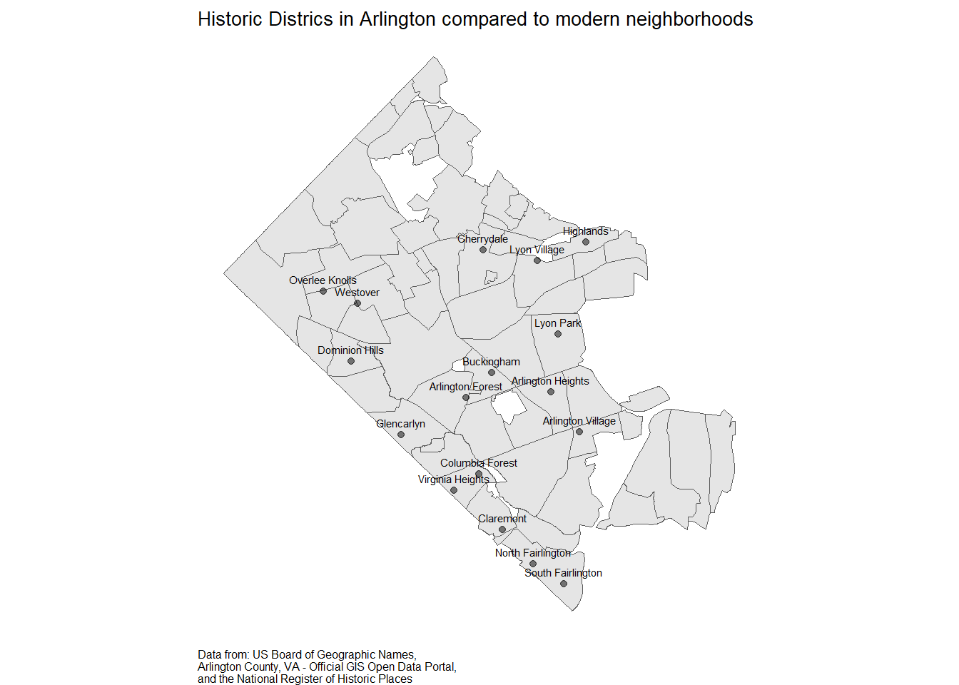
Today’s TidyTuesday is about place names as recorded by the US Board on Geographic Names. The dataset has been cleaned to include only populated places. This week will involve more libraries than normal, since I am going to play with mapping. library(tidyverse) # who doesn't want to be tidy? ...

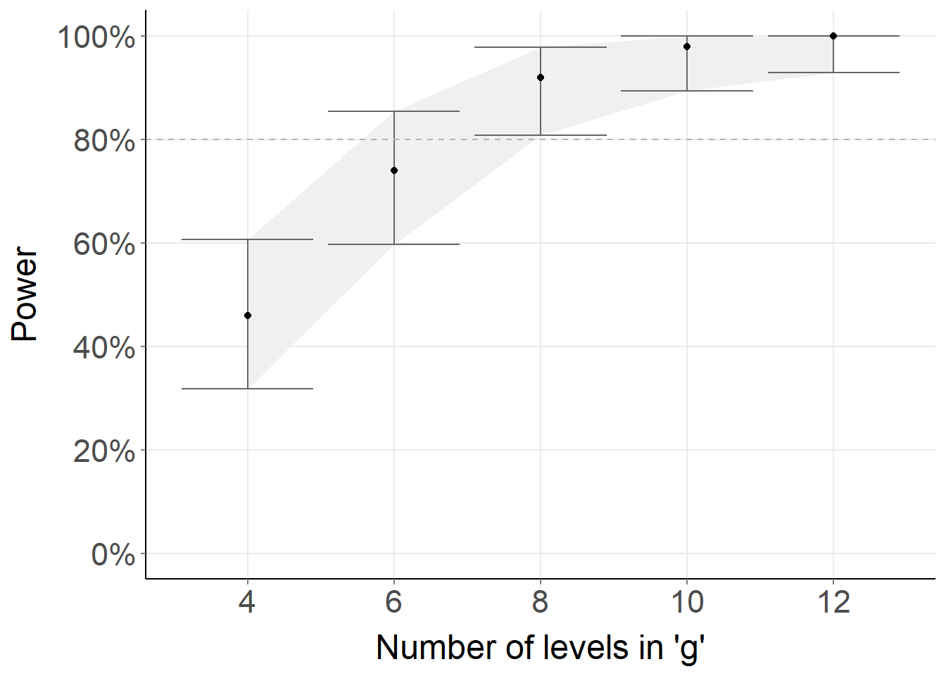
The R package simr has greatly facilitated power analysis for mixed-effects models using Monte Carlo simulation (i.e., hundreds or thousands of tests under slight variations of the data). The powerCurve function is used to estimate the statistical power for various sample sizes in one go. Since it runs serially, ...

Mustafa Cavus, organizer of the Eskisehir R User Group, in Turkey, discussed the diverse and thriving R community in Eskisehir. He shared the details of a 4-day event hosted by... The post R for Predictive Modeling and Data Visualization in Turkey appeared first on R Consortium.

Introduction Welcome to the world of data visualization in R! In this blog post, we will explore the abline() function, a versatile tool that allows you to add straight lines to your plots effortlessly. Whether you’re a beginner or an experience...

Over a year ago, while listing to a very not-at-all-statistical podcast, I discovered that Bayesian modeling is widely used in archaeology since the mid 90s to calibrate carbon dating.1 Carbon dating is a scientific method used to determine the a...

Whereas the direction of main effects can be interpreted from the sign of the estimate, the interpretation of interaction effects often requires plots. This task is facilitated by the R package sjPlot (Lüdecke, 2022). For instance, using the plot_model function, I plotted the interaction between two continuous variables.

library(lme4)
#> Loading required package: Matrix
library(sjPlot)
#> Learn more about sjPlot with 'browseVignettes("sjPlot")'.
library(ggplot2)

theme_set(theme_sjplot())

# Create data partially based on code by Ben Bolker  
# from https://stackoverflow.com/a/38296264/7050882

set.seed(101)

spin = runif(800, 1, 24)

trait = rep(1:40, each = 20)

ID = rep(1:80, each = 10)

testdata <- data.frame(spin, trait, ID)

testdata$fatigue <- 
  testdata$spin * testdata$trait / 
  rnorm(800, mean = 6, sd = 2)

# Model
fit = lmer(fatigue ~ spin * trait + (1|ID),
           data = testdata, REML = TRUE)
#> boundary (singular) fit: see help('isSingular')

plot_model(fit, type = 'pred', terms = c('spin', 'trait'))
#> Warning: Ignoring unknown parameters: linewidth

...

Whereas the direction of main effects can be interpreted from the sign of the estimate, the interpretation of interaction effects often requires plots. This task is facilitated by the R package sjPlot (Lüdecke, 2022). For instance, using the plot_model function, I plotted the interaction between two continuous variables.

library(lme4)
#> Loading required package: Matrix
library(sjPlot)
library(ggplot2)

theme_set(theme_sjplot())

# Create data using code by Ben Bolker from 
# https://stackoverflow.com/a/38296264/7050882

set.seed(101)
spin = runif(600, 1, 24)
reg = runif(600, 1, 15)
ID = rep(c("1","2","3","4","5", "6", "7", "8", "9", "10"))
day = rep(1:30, each = 10)
testdata <- data.frame(spin, reg, ID, day)
testdata$fatigue <- testdata$spin * testdata$reg/10 * rnorm(30, mean=3, sd=2)

fit = lmer(fatigue ~ spin * reg + (1|ID),
           data = testdata, REML = TRUE)

plot_model(fit, type = 'pred', terms = c('spin', 'reg'))
#> Warning: Ignoring unknown parameters: linewidth

...

Whereas the direction of main effects can be interpreted from the sign of the estimate, the interpretation of interaction effects often requires plots. This task is facilitated by the R package sjPlot (Lüdecke, 2022). For instance, using the plot_model function, I plotted the interaction between a continuous variable and ...

To assess whether convergence warnings render the results invalid, or on the contrary, the results can be deemed valid in spite of the warnings, Bates et al. (2023) suggest refitting models affected by convergence warnings with a variety of optimizers. The authors argue that, if the different optimizers produce practically-equivalent results, ...

R and Shiny Training: If you find this blog to be interesting, please note that I offer personalized and group-based training sessions that may be reserved through Buy me a Coffee. Additionally, I provide training services in the Spanish language ...