Boosting Win Probability accuracy with player embeddings
Want to share your content on R-bloggers? click here if you have a blog, or here if you don't.
In my previous post Computing Win Probability of T20 matches I had discussed various approaches on computing Win Probability of T20 matches. I had created ML models with glmnet and random forest using TidyModels. This was what I had achieved
- glmnet : accuracy – 0.67 and sensitivity/specificity – 0.68/0.65
- random forest : accuracy – 0.737 and roc_auc- 0.834
- DL model with Keras in Python : accuracy – 0.73
I wanted to see if the performance of the models could be further improved. I got a suggestion from a AI/DL whizkid, who is close to me, to include embeddings for batsmen and bowlers. He felt that win percentage is influenced by which batsman faces which bowler.
So, I started to explore this idea. Embeddings can be used to convert categorical variables to a vector of continuous floating point numbers.Fortunately R’s Tidymodels, has a convenient functionality to create embeddings. By including embeddings for batsman, bowler the performance of my ML models improved vastly. Now the performance is
- glmnet : accuracy – 0.728 and roc_auc – 0.81
- random forest : accuracy – 0.927 and roc_auc – 0.98
- mlp-dnn :accuracy – 0.762 and roc_auc – 0.854
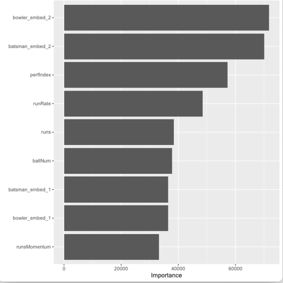
As can be seem there is almost a 20% increase in accuracy with random forests with embeddings over the model without embeddings. Moreover, the feature importance which is plotted below shows that the bowler and batsman embeddings have a significant influence on the Win Probability
Note: The data for this analysis is taken from Cricsheet and has been processed with my R package yorkr.
A. Win Probability using GLM with penalty and player embeddings
Here Generalised Linear Model (GLMNET) for Logistic Regression is used. In the GLMNET the regularisation path is computed for the lasso or elastic net penalty at a grid of values for the regularisation parameter lambda. glmnet is extremely fast and gave an accuracy of 0.72 for an roc_auc of 0.81 with batsman, bowler embeddings. This was good improvement over my earlier implementation with glmnet without the batsman & bowler embeddings which had a
- Read the data
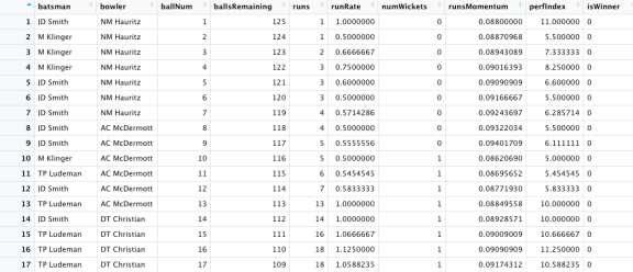
a) Read the data from 9 T20 leagues (BBL, CPL, IPL, NTB, PSL, SSM, T20 Men, T20 Women, WBB) and create a single data frame of ball-by-ball data. Display the data frame
library(dplyr)
library(caret)
library(e1071)
library(ggplot2)
library(tidymodels)
library(embed)

# Helper packages
library(readr)       # for importing data
library(vip)

df1=read.csv("output3/matchesBBL3.csv")
df2=read.csv("output3/matchesCPL3.csv")
df3=read.csv("output3/matchesIPL3.csv")
df4=read.csv("output3/matchesNTB3.csv")
df5=read.csv("output3/matchesPSL3.csv")
df6=read.csv("output3/matchesSSM3.csv")
df7=read.csv("output3/matchesT20M3.csv")
df8=read.csv("output3/matchesT20W3.csv")
df9=read.csv("output3/matchesWBB3.csv")

#Bind all dataframes together
df=rbind(df1,df2,df3,df4,df5,df6,df7,df8,df9)
glimpse(df)
Rows: 1,199,115
Columns: 10
$ batsman        <chr> "JD Smith", "M Klinger", "M Klinger", "M Klinger", "JD …
$ bowler         <chr> "NM Hauritz", "NM Hauritz", "NM Hauritz", "NM Hauritz",…

$ ballNum        <int> 1, 2, 3, 4, 5, 6, 7, 8, 9, 10, 11, 12, 13, 14, 15, 16, …
$ ballsRemaining <int> 125, 124, 123, 122, 121, 120, 119, 118, 117, 116, 115, …
$ runs           <int> 1, 1, 2, 3, 3, 3, 4, 4, 5, 5, 6, 7, 13, 14, 16, 18, 18,…

$ runRate        <dbl> 1.0000000, 0.5000000, 0.6666667, 0.7500000, 0.6000000, …
$ numWickets     <int> 0, 0, 0, 0, 0, 0, 0, 0, 0, 1, 1, 1, 1, 1, 1, 1, 1, 1, 1…
$ runsMomentum   <dbl> 0.08800000, 0.08870968, 0.08943089, 0.09016393, 0.09090…
$ perfIndex      <dbl> 11.000000, 5.500000, 7.333333, 8.250000, 6.600000, 5.50…
$ isWinner       <int> 0, 0, 0, 0, 0, 0, 0, 0, 0, 0, 0, 0, 0, 0, 0, 0, 0, 0, 0…


df %>%
  count(isWinner) %>%
  mutate(prop = n/sum(n))
  isWinner      n      prop
1
0 614237 0.5122419
2
1 584878 0.4877581
2) Create training.validation and test sets
b) Split to training, validation and test sets. The dataset is initially split into training and test in the ratio 80%:20%. The training data is again split into training and validation in the ratio 80:20
set.seed(123)
splits      <- initial_split(df,prop = 0.80)
splits
<Training/Testing/Total>
<959292/239823/1199115>
df_other <- training(splits)
df_test  <- testing(splits)

set.seed(234)
val_set <- validation_split(df_other,prop = 0.80)
val_set
# A tibble: 1 × 2
  splits
id
  <list>                  <chr>
1 <split [767433/191859]> validation
3) Create pre-processing recipe
a) Normalise the following predictors
- ballNum
- ballsRemaining
- runs
- runRate
- numWickets
- runsMomentum
- perfIndex
b) Create floating point embeddings for
- batsman
- bowler
4) Create a Logistic Regression Workflow by adding the GLM model and the recipe
5) Create grid of elastic penalty values for regularisation
6) Train all 30 models
7) Plot the ROC of the model against the penalty
# Use all 12 cores
cores <- parallel::detectCores()
cores
# Create a Logistic Regression model with penalty
lr_mod <-
  logistic_reg(penalty = tune(), mixture = 1) %>%
  set_engine("glmnet",num.threads = cores)

# Create pre-processing recipe
lr_recipe <-
  recipe(isWinner ~ ., data = df_other) %>%
  step_embed(batsman,bowler, outcome = vars(isWinner)) %>%  step_normalize(ballNum,ballsRemaining,runs,runRate,numWickets,runsMomentum,perfIndex)

# Set the workflow by adding the GLM model with the recipe
lr_workflow <-
  workflow() %>%
  add_model(lr_mod) %>%
  add_recipe(lr_recipe)

# Create a grid for the elastic net penalty
lr_reg_grid <- tibble(penalty = 10^seq(-4, -1, length.out = 30))
lr_reg_grid %>% top_n(-5)
# A tibble: 5 × 1
   penalty

<dbl>
1 0.0001
2 0.000127
3 0.000161
4 0.000204
5 0.000259

lr_reg_grid %>% top_n(5)  # highest penalty values
# A tibble: 5 × 1
  penalty
    <dbl>
1  0.0386
2  0.0489
3  0.0621
4  0.0788
5  0.1

# Train 30 penalized models
lr_res <-
  lr_workflow %>%
  tune_grid(val_set,
            grid = lr_reg_grid,
            control = control_grid(save_pred = TRUE),
            metrics = metric_set(accuracy,roc_auc))

# Plot the penalty versus ROC
lr_plot <-
  lr_res %>%
  collect_metrics() %>%
  ggplot(aes(x = penalty, y = mean)) +
  geom_point() +
  geom_line() +
  ylab("Area under the ROC Curve") +
  scale_x_log10(labels = scales::label_number())

lr_plot
The Penalty vs ROC plot is shown below

8) Display the ROC_AUC of the top models with the penalty
9) Select the model with the best ROC_AUC and the associated penalty. It can be seen the best mean ROC_AUC is 0.81 and the associated penalty is 0.000530
top_models <-
  lr_res %>%
  show_best("roc_auc", n = 15) %>%
  arrange(penalty)
top_models

# A tibble: 15 × 7
    penalty .metric .estimator  mean     n std_err .config
      <dbl> <chr>   <chr>      <dbl> <int>   <dbl> <chr>
 1 0.0001   roc_auc binary     0.810     1      NA Preprocessor1_Model01
 2 0.000127 roc_auc binary     0.810     1      NA Preprocessor1_Model02
 3 0.000161 roc_auc binary     0.810     1      NA Preprocessor1_Model03
 4 0.000204 roc_auc binary     0.810     1      NA Preprocessor1_Model04
 5 0.000259 roc_auc binary     0.810     1      NA Preprocessor1_Model05
 6 0.000329 roc_auc binary     0.810     1      NA Preprocessor1_Model06
 7 0.000418 roc_auc binary     0.810     1      NA Preprocessor1_Model07
 8 0.000530 roc_auc binary     0.810     1      NA Preprocessor1_Model08
 9 0.000672 roc_auc binary     0.810     1      NA Preprocessor1_Model09
10 0.000853 roc_auc binary     0.810     1      NA Preprocessor1_Model10
11 0.00108  roc_auc binary     0.810     1      NA Preprocessor1_Model11
12 0.00137  roc_auc binary     0.810     1      NA Preprocessor1_Model12
13 0.00174  roc_auc binary     0.809     1      NA Preprocessor1_Model13
14 0.00221  roc_auc binary     0.809     1      NA Preprocessor1_Model14
15 0.00281  roc_auc binary     0.809     1      NA Preprocessor1_Model15

#Picking the best model and the corresponding penalty
lr_best <-
  lr_res %>%
  collect_metrics() %>%
  arrange(penalty) %>%
  slice(8)
lr_best
# A tibble: 1 × 7

   penalty .metric .estimator  mean     n std_err .config
     <dbl> <chr>   <chr>      <dbl> <int>   <dbl> <chr>

1 0.000530 roc_auc binary     0.810     1      NA Preprocessor1_Model08

# Collect predictions and generate the AUC curve
lr_auc <-
  lr_res %>%
  collect_predictions(parameters = lr_best) %>%
  roc_curve(isWinner, .pred_0) %>%
  mutate(model = "Logistic Regression")

autoplot(lr_auc)
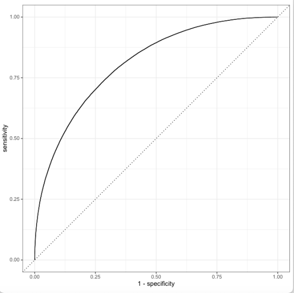
7) Plot the Area under the Curve (AUC).
10) Build the final model with the best LR parameters value as found in lr_best
a) The best performance was for a penalty of 0.000530
b) The accuracy achieved is 0.72. Clearly using the embeddings for batsman, bowlers improves on the performance of the GLM model without the embeddings. The accuracy achieved was 0.72 whereas previously it was 0.67 see (Computing Win Probability of T20 Matches)
c) Create a fit with the best parameters
d) The accuracy is 72.8% and the ROC_AUC is 0.813
# Create a model with the penalty for best ROC_AUC
last_lr_mod <-
  logistic_reg(penalty = 0.000530, mixture = 1) %>%
  set_engine("glmnet",num.threads = cores,importance = "impurity")

#Update the workflow with this model
last_lr_workflow <-
  lr_workflow %>%
  update_model(last_lr_mod)

#Create a fit
set.seed(345)
last_lr_fit <-
  last_lr_workflow %>%
  last_fit(splits)

#Generate accuracy, roc_auc
last_lr_fit %>%
  collect_metrics()
# A tibble: 2 × 4
  .metric  .estimator .estimate .config

<chr>    <chr>          <dbl> <chr>
1 accuracy binary         0.728 Preprocessor1_Model1

2 roc_auc  binary         0.813 Preprocessor1_Model1
11) Plot the feature importance
It can be seen that bowler and batsman embeddings are the most significant for the prediction followed by runRate.
runRate –
- runRate in 1st innings
- requiredRunRate in 2nd innings

12) Plot the ROC characteristics
last_lr_fit %>%
  collect_predictions() %>%
  roc_curve(isWinner, .pred_0) %>%
  autoplot()

13) Generate a confusion matrix
14) Create a final Generalised Linear Model for Logistic Regression with the penalty of 0.000530
15) Save the model
# generate predictions from the test set
test_predictions <- last_lr_fit %>% collect_predictions()
test_predictions

# generate a confusion matrix
test_predictions %>%
  conf_mat(truth = isWinner, estimate = .pred_class)

Truth
Prediction     0     1

0                  90105 32658

1                  32572 84488

final_lr_model <- fit(last_lr_workflow, df_other)

final_lr_model

obj_size(final_lr_model)
146.51 MB


butcher::weigh(final_lr_model)
A tibble: 305 × 2
object                                  size
<chr>                                  <dbl>
  1 pre.actions.recipe.recipe.steps.terms1  57.9
2 pre.actions.recipe.recipe.steps.terms2  57.9
3 pre.actions.recipe.recipe.steps.terms3  57.9


cleaned_lm <- butcher::axe_env(final_lr_model, verbose = TRUE)
#✔ Memory released: "1.04 kB"
#✔ Memory released: "1.62 kB"

saveRDS(cleaned_lm, "cleanedLR.rds")
16) Compute Ball-by-ball Win Probability
- Chennai Super Kings-Lucknow Super Giants-2022-03-31
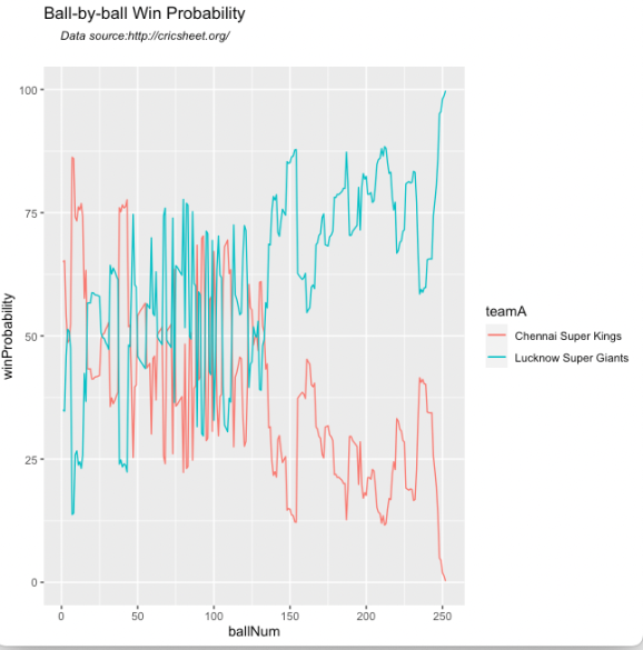
16a) The corresponding Worm-wicket graph for this match is as below
- Chennai Super Kings-Lucknow Super Giants-2022-03-31

B) Win Probability using Random Forest with player embeddings
In the 2nd approach I use Random Forest with batsman and bowler embeddings. The performance of the model with embeddings is quantum jump from the earlier performance without embeddings. However, the random forest is also computationally intensive.
1) Read the data
a) Read the data from 9 T20 leagues (BBL, CPL, IPL, NTB, PSL, SSM, T20 Men, T20 Women, WBB) and create a single data frame of ball-by-ball data. Display the data frame
2) Create training.validation and test sets
b) Split to training, validation and test sets. The dataset is initially split into training and test in the ratio 80%:20%. The training data is again split into training and validation in the ratio 80:20
library(dplyr)
library(caret)
library(e1071)
library(ggplot2)
library(tidymodels)
library(tidymodels)
library(embed)

# Helper packages
library(readr)       # for importing data
library(vip)
library(ranger)

# Read all the 9 T20 leagues
df1=read.csv("output3/matchesBBL3.csv")
df2=read.csv("output3/matchesCPL3.csv")
df3=read.csv("output3/matchesIPL3.csv")
df4=read.csv("output3/matchesNTB3.csv")
df5=read.csv("output3/matchesPSL3.csv")
df6=read.csv("output3/matchesSSM3.csv")
df7=read.csv("output3/matchesT20M3.csv")
df8=read.csv("output3/matchesT20W3.csv")
df9=read.csv("output3/matchesWBB3.csv")

# Bind into a single dataframe
df=rbind(df1,df2,df3,df4,df5,df6,df7,df8,df9)

set.seed(123)
df$isWinner = as.factor(df$isWinner)

#Split data into training, validation and test sets
splits      <- initial_split(df,prop = 0.80)
df_other <- training(splits)
df_test  <- testing(splits)
set.seed(234)
val_set <- validation_split(df_other, prop = 0.80)
val_set
2) Create a Random Forest model tuning for number of predictor nodes at each decision node (mtry) and minimum number of predictor nodes (min_n)
3) Use the ranger engine and set up for classification
4) Set up the recipe and include batsman and bowler embeddings
5) Create a workflow and add the recipe and the random forest model with the tuning parameters
# Use all 12 cores parallely
cores <- parallel::detectCores()
cores
[1] 12

# Create the random forest model with mtry and min as tuning parameters
rf_mod <-
  rand_forest(mtry = tune(), min_n = tune(), trees = 1000) %>%
  set_engine("ranger", num.threads = cores) %>%
  set_mode("classification")

# Setup the recipe with batsman and bowler embeddings
rf_recipe <-
  recipe(isWinner ~ ., data = df_other) %>%
  step_embed(batsman,bowler, outcome = vars(isWinner))

# Create the random forest workflow
rf_workflow <-
  workflow() %>%
  add_model(rf_mod) %>%
  add_recipe(rf_recipe)

rf_mod
# show what will be tuned
extract_parameter_set_dials(rf_mod)

set.seed(345)
# specify which values meant to tune

# Build the model
rf_res <-
  rf_workflow %>%
  tune_grid(val_set,
            grid = 10,
            control = control_grid(save_pred = TRUE),
            metrics = metric_set(accuracy,roc_auc))

# Pick the best  roc_auc and the associated tuning parameters
rf_res %>%
  show_best(metric = "roc_auc")
# A tibble: 5 × 8
   mtry min_n .metric .estimator  mean     n std_err .config
  <int> <int> <chr>   <chr>      <dbl> <int>   <dbl> <chr>
1     4     4 roc_auc binary     0.980     1      NA Preprocessor1_Model08
2     9     8 roc_auc binary     0.979     1      NA Preprocessor1_Model03

3     8    16 roc_auc binary     0.974     1      NA Preprocessor1_Model10
4     7    22 roc_auc binary     0.969     1      NA Preprocessor1_Model09

5     5    19 roc_auc binary     0.969     1      NA Preprocessor1_Model06

rf_res %>%
  show_best(metric = "accuracy")
# A tibble: 5 × 8

mtry min_n .metric  .estimator  mean     n std_err .config
  <int> <int> <chr>    <chr>      <dbl> <int>   <dbl> <chr>
1  4     4 accuracy binary    0.927     1      NA Preprocessor1_Model08

2  9     8 accuracy binary    0.926     1      NA Preprocessor1_Model03
3  8    16 accuracy binary    0.915     1      NA Preprocessor1_Model10
4  7    22 accuracy binary    0.906     1      NA Preprocessor1_Model09

5  5    19 accuracy binary    0.904     1      NA Preprocessor1_Model0
6) Select all models with the best roc_auc. It can be seen that the best roc_auc is 0.980 for mtry=4 and min_n=4
7) Get the model with the highest accuracy. The highest accuracy achieved is 0.927 or 92.7. This accuracy is also for mtry=4 and min_n=4
# Pick the best  roc_auc and the associated tuning parameters
rf_res %>%
  show_best(metric = "roc_auc")
# A tibble: 5 × 8
   mtry min_n .metric .estimator  mean     n std_err .config
  <int> <int> <chr>   <chr>      <dbl> <int>   <dbl> <chr>
1     4     4 roc_auc binary     0.980     1      NA Preprocessor1_Model08
2     9     8 roc_auc binary     0.979     1      NA Preprocessor1_Model03

3     8    16 roc_auc binary     0.974     1      NA Preprocessor1_Model10
4     7    22 roc_auc binary     0.969     1      NA Preprocessor1_Model09

5     5    19 roc_auc binary     0.969     1      NA Preprocessor1_Model06

# Display the accuracy of the models in descending order and the parameters
rf_res %>%
  show_best(metric = "accuracy")
# A tibble: 5 × 8

mtry min_n .metric  .estimator  mean     n std_err .config
  <int> <int> <chr>    <chr>      <dbl> <int>   <dbl> <chr>
1  4     4 accuracy binary    0.927     1      NA Preprocessor1_Model08

2  9     8 accuracy binary    0.926     1      NA Preprocessor1_Model03
3  8    16 accuracy binary    0.915     1      NA Preprocessor1_Model10
4  7    22 accuracy binary    0.906     1      NA Preprocessor1_Model09

5  5    19 accuracy binary    0.904     1      NA Preprocessor1_Model0
8) Select the model with the best parameters for accuracy mtry=4 and min_n=4. For this the accuracy is 0.927. For this configuration the roc_auc is also the best at 0.980
9) Plot the Area Under the Curve (AUC). It can be seen that this model performs really well and it hugs the top left.
# Pick the best model
rf_best <-
  rf_res %>%
  select_best(metric = "accuracy")

# The best model has mtry=4 and min=4
rf_best
     mtry min_n .config
  <int> <int> <chr>
1     4     4      Preprocessor1_Model08

#Plot AUC
rf_auc <-
  rf_res %>%
  collect_predictions(parameters = rf_best) %>%
  roc_curve(isWinner, .pred_0) %>%
  mutate(model = "Random Forest")

autoplot(rf_auc)

10) Create the final model with the best parameters
11) Execute the final fit
12) Plot feature importance, The bowler and batsman embedding followed by perfIndex and runRate are features that contribute the most to the Win Probability
last_rf_mod <-
  rand_forest(mtry = 4, min_n = 4, trees = 1000) %>%
  set_engine("ranger", num.threads = cores, importance = "impurity") %>%
  set_mode("classification")

# the last workflow
last_rf_workflow <-
  rf_workflow %>%
  update_model(last_rf_mod)

set.seed(345)
last_rf_fit <-
  last_rf_workflow %>%
  last_fit(splits)

last_rf_fit %>%
  collect_metrics()

  .metric  .estimator .estimate .config
  <chr>    <chr>          <dbl> <chr>

1 accuracy binary         0.944 Preprocessor1_Model1
2 roc_auc  binary         0.988 Preprocessor1_Model1

last_rf_fit %>%
  extract_fit_parsnip() %>%
  vip(num_features = 9)
13) Plot the ROC curve for the best fit
# Plot the ROC for the final model
last_rf_fit %>%
  collect_predictions() %>%
  roc_curve(isWinner, .pred_0) %>%
  autoplot()
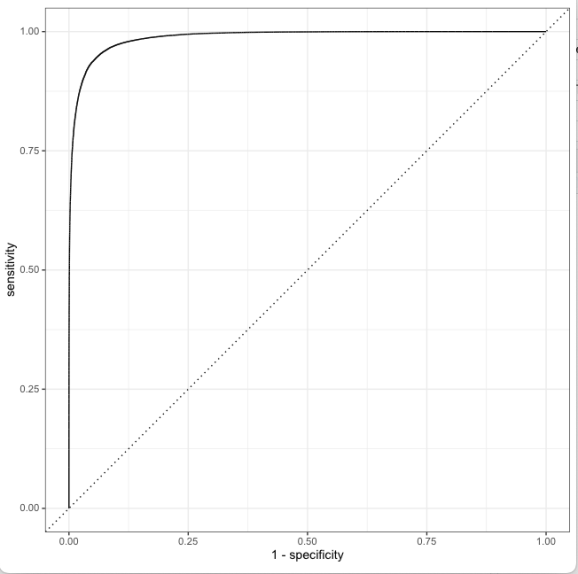
14) Create a confusion matrix
We can see that the number of false positives and false negatives is very low
15) Create the final fit with the Random Forest Model
# generate predictions from the test set
test_predictions <- last_rf_fit %>% collect_predictions()
test_predictions

   id               .pred_0 .pred_1  .row .pred_class isWinner .config
   <chr>              <dbl>   <dbl> <int> <fct>       <fct>    <chr>
 1 train/test split   0.838  0.162      1 0           0       Preprocessor1_Mo…
 2
train/test split   0.463  0.537     11 1           0        Preprocessor1_Mo…
 3
train/test split   0.846  0.154     14 0           0        Preprocessor1_Mo…
 4
train/test split   0.839  0.161     22 0           0        Preprocessor1_Mo…
 5
train/test split   0.846  0.154     36 0           0        Preprocessor1_Mo…
 6
train/test split   0.848  0.152     37 0           0        Preprocessor1_Mo…
 7
train/test split   0.731  0.269     39 0           0        Preprocessor1_Mo…
 8
train/test split   0.972  0.0281    40 0           0        Preprocessor1_Mo…
 9
train/test split   0.655  0.345     42 0           0        Preprocessor1_Mo…
10
train/test split   0.662  0.338     43 0           0        Preprocessor1_Mo…

# generate a confusion matrix
test_predictions %>%
  conf_mat(truth = isWinner, estimate = .pred_class)

          Truth
Prediction      0      1

          0 116576   7096

          1   6391 109760

# Create the final model
final_model <- fit(last_rf_workflow, df_other)
16) Computing Win Probability with Random Forest Model for match
- Pakistan-India-2022-10-23

17) Worm -wicket graph of match
- Pakistan-India-2022-10-23

C) Win Probability using MLP – Deep Neural Network (DNN) with player embeddings
In this approach the MLP package of Tidymodels was used. Multi-layer perceptron (MLP) with Deep Neural Network (DNN) was used to compute the Win Probability using player embeddings. An accuracy of 0.76 was obtained
1) Read the data
a) Read the data from 9 T20 leagues (BBL, CPL, IPL, NTB, PSL, SSM, T20 Men, T20 Women, WBB) and create a single data frame of ball-by-ball data. Display the data frame
2) Create training.validation and test sets
b) Split to training, validation and test sets. The dataset is initially split into training and test in the ratio 80%:20%. The training data is again split into training and validation in the ratio 80:20
library(dplyr)
library(caret)
library(e1071)
library(ggplot2)
library(tidymodels)
library(embed)

# Helper packages
library(readr)       # for importing data
library(vip)
library(ranger)

df1=read.csv("output3/matchesBBL3.csv")
df2=read.csv("output3/matchesCPL3.csv")
df3=read.csv("output3/matchesIPL3.csv")
df4=read.csv("output3/matchesNTB3.csv")
df5=read.csv("output3/matchesPSL3.csv")
df6=read.csv("output3/matchesSSM3.csv")
df7=read.csv("output3/matchesT20M3.csv")
df8=read.csv("output3/matchesT20W3.csv")
df9=read.csv("output3/matchesWBB3.csv")

df=rbind(df1,df2,df3,df4,df5,df6,df7,df8,df9)


set.seed(123)
df$isWinner = as.factor(df$isWinner)
splits      <- initial_split(df,prop = 0.80)
df_other <- training(splits)
df_test  <- testing(splits)
set.seed(234)
val_set <- validation_split(df_other,
                            prop = 0.80)
val_set
3) Create a Deep Neural Network recipe
- Normalize parameters
- Add embeddings for batsman, bowler
4) Set the MLP-DNN hyperparameters
- epochs=100
- hidden units =5
- dropout regularization =0.1
5) Fit on Training data
cores <- parallel::detectCores()
cores

nn_recipe <-
  recipe(isWinner ~ ., data = df_other) %>%
step_normalize(ballNum,ballsRemaining,runs,runRate,numWickets,runsMomentum,perfIndex) %>%
  step_embed(batsman,bowler, outcome = vars(isWinner)) %>%
  prep(training = df_other, retain = TRUE)

# For validation:
test_normalized <- bake(nn_recipe, new_data = df_test)

set.seed(57974)
# Set the hyper parameters for DNN
# Use Keras
# Fit on training data
nnet_fit <-
  mlp(epochs = 100, hidden_units = 5, dropout = 0.1) %>%
  set_mode("classification") %>%
  # Also set engine-specific `verbose` argument to prevent logging the results:
  set_engine("keras", verbose = 0) %>%
  fit(isWinner ~ ., data = bake(nn_recipe, new_data = df_other))

nnet_fit
parsnip model object
Model:"sequential"

____________________________________________________________________________

Layer (type)                                           Output Shape                                    Param #
============================================================================
dense (Dense)                                           (None, 5)                                          60
____________________________________________________________________________

dense_1 (Dense)                                         (None, 5)                                          30
____________________________________________________________________________
dropout (Dropout)                                       (None, 5)                                          0
____________________________________________________________________________
dense_2 (Dense)                                         (None, 2)                                          12
============================================================================
Total params: 102
Trainable params: 102
Non-trainable params: 0
6) Test on Test data
- Check ROC_AUC. It is 0.854
- Check accuracy. The MLP-DNN gives a decent performance with an acuracy of 0.76
- Compute the Confusion Matrix
# Validate on test data
val_results <-
  df_test %>%
  bind_cols(
    predict(nnet_fit, new_data = test_normalized),
    predict(nnet_fit, new_data = test_normalized, type = "prob")
  )
val_results

# Check roc_auc
val_results %>% roc_auc(truth = isWinner, .pred_0)
  .metric .estimator .estimate

   <chr>   <chr>          <dbl>
1 roc_auc binary         0.854

# Check accuracy
val_results %>% accuracy(truth = isWinner, .pred_class)
  .metric  .estimator .estimate
  <chr>    <chr>          <dbl>
1 accuracy binary         0.762

# Display confusion matrix
val_results %>% conf_mat(truth = isWinner, .pred_class)
          Truth
Prediction
           0     1
       0 97419 31564
       1 25548 85292
Conclusion
- Of the 3 ML models, glmnet, random forest and Multi-layer Perceptron DNN, random forest had the best performance
- Random Forest ML model with batsman, bowler embeddings was able to achieve an accuracy of 92.4% and a ROC_AUC of 0.98 with very low false positives, negatives. This was a quantum jump from my earlier random forest model without embeddings which had an accuracy of 73.7% and an ROC_AUC of 0.834
- The glmnet and NN models are fairly light weight. Random Forest is computationally very intensive.
Check out my other posts
- Using Reinforcement Learning to solve Gridworld
- Deep Learning from first principles in Python, R and Octave – Part 8
- Introducing QCSimulator: A 5-qubit quantum computing simulator in R
- Big Data-5: kNiFi-ing through cricket data with yorkpy
- Singularity
- Practical Machine Learning with R and Python – Part 6
- GooglyPlusPlus2022 optimizes batting/bowling lineup
- Fun simulation of a Chain in Android
- Introducing cricpy:A python package to analyze performances of cricketers
- Programming languages in layman’s language
To see all posts click Index of posts
R-bloggers.com offers daily e-mail updates about R news and tutorials about learning R and many other topics. Click here if you're looking to post or find an R/data-science job.
Want to share your content on R-bloggers? click here if you have a blog, or here if you don't.
