
Regime Switching State Space Model with R code
[This article was first published on K & L Fintech Modeling, and kindly contributed to R-bloggers]. (You can report issue about the content on this page here)
Want to share your content on R-bloggers? click here if you have a blog, or here if you don't.
This post explains a Markov regime switching state space model. The bottom line is two-fold: 1) expanding states by each regime transitions and 2) collapsing each updated estimates for the next state prediction. The step 2) is necessary to fix the dimension of previous states so that Kalman recursion does not produce exponentially increasing states. This combined filter is called Kim filter (= Kalman filter + Hamilton filter + Kim collapsing procedure). Want to share your content on R-bloggers? click here if you have a blog, or here if you don't.
Regime Switching State Space Model
In the previous posts below, we have explained and implemented regime switching models.
In this post, to complete a series of posts regarding the regime switching model, a regime switching state space model is investigated. The content of this post is heavily borrowed from Kim (1994) and Kim and Nelson (1999).
Regime Switching State Space Model
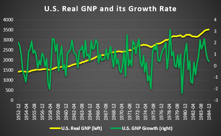
As an example of a regime switching state space model, Prof. Kim used the following generalized Hamilton model for the log of real GNP (Lam; 1990) in his paper and book.
\[\begin{align} \ln(GNP_t) &= n_t + x_t \\ n_t &= n_{t-1} + \mu_0 + \mu_1 s_t \\ x_t &= \phi_1 x_{t-1} + \phi_2 x_{t-2} + u_t \\ \\ u_t &\sim N(0,\sigma^2) \\ s_t &= 0,1 \quad P_{ij} = \begin{bmatrix} p_{00} & p_{01} \\ p_{10} & p_{11} \end{bmatrix} \end{align}\]
where \(\ln(GNP_t)\) is a real GNP level. \(n_t\) is a deterministic series with a regime-switching growth rate and \(x_t\) is stationary AR(2) cycle process.
Since \(\ln(GNP_t)\) is the log level variable, the difference of it, \(y_t = \ln(GNP_t)-\ln(GNP_{t-1})\), can be represented as a state space model in the following way.
\[\begin{align} y_t &= \mu_0 + \mu_1 s_t + x_t-x_{t-1} \\ x_t &= \phi_1 x_{t-1} + \phi_2 x_{t-2} + u_t \end{align}\]
It is a typical approach that a state space model is represented as a vector-matrix form for using Kalman filter as follows.
\[\begin{align} y_t &= \mu_{s_t} + \begin{bmatrix} 1 & -1 \end{bmatrix} \begin{bmatrix} x_{t} \\ x_{t-1} \end{bmatrix} \\ \begin{bmatrix} x_t \\ x_{t-1} \end{bmatrix} &= \begin{bmatrix} \phi_1 & \phi_2 \\ 1 & 0 \end{bmatrix} \begin{bmatrix} x_{t-1} \\ x_{t-2} \end{bmatrix} +\begin{bmatrix} u_{t} \\ 0 \end{bmatrix} \\ \\ u_t &\sim N(0,\sigma^2) \\ \mu_{s_t} &= \mu_0 + \mu_1 s_t,\quad \mu_1 \gt 0 \\ s_t &= 0,1 \quad P_{ij} = \begin{bmatrix} p_{00} & p_{01} \\ p_{10} & p_{11} \end{bmatrix} \\ & \quad \quad \Downarrow \\ \color{blue}{y_t} & \color{blue}{= \mu_{s_t} + F \mathbf{x}_t} \\ \color{blue}{\mathbf{x}_t} & \color{blue}{= A \mathbf{x}_{t-1} + v_t} \end{align}\]
For the sake of notational simplicity, we use \(x_t\) instead of \(\mathbf{x}_t\).
Kalman Filtering
Kalman filter with regime switching is used to get state estimates from a state space model taking regime transition into account and has the following recursion.
\[\begin{align} x_{t|t-1}^{ij} &= Ax_{t-1|t-1}^i \\ P_{t|t-1}^{ij} &= AP_{t-1|t-1}^i A^{T} + Q \\ \eta_{t|t-1}^{ij} &= y_t – \mu_j – Fx_{t|t-1}^{ij} \\ H_{t|t-1}^{ij} &= F P_{t|t-1}^{ij} F^{T} + R \\ K^{ij} &= P_{t|t-1}^{ij}F^{T}[H_{t|t-1}^{ij}]^{-1} \\ x_{t|t}^{ij} &= x_{t|t-1}^{ij} + K^{ij} \eta_{t|t-1}^{ij} \\ P_{t|t}^{ij} &= (I – K^{ij} F) P_{t|t-1}^{ij} \end{align}\]
In regime-dependent Kalman filter, all the notations are augmented with superscript \(\{ij\}\) except \(x_{t-1|t-1}^i\) and \(P_{t-1|t-1}^i\) since these two estimates are in i-state (two-state) but other estimates must reflect state transitions from i to j (four-state). For example, \(x_{t|t-1}\) and \(x_{t|t-1}^{ij}\) are different in terms of conditioning information.
\[\begin{align} x_{t|t-1} &= E[X_t|\psi_{t-1}] \\ x_{t|t-1}^{ij} &= E[X_t|\psi_{t-1}, S_t=j, S_{t-1}=i] \end{align}\]
In contrast to the single regime, however, in the multiple regimes, \(x_{t|t}^{ij}\) and \(P_{t|t}^{ij}\) cannot be used the next state prediction due simply to the mismatch both 1) between \(x_{t|t}^{ij}\) and \(x_{t-1|t-1}^i\) and 2) between \(P_{t|t}^{ij}\) and \(P_{t-1|t-1}^i\). To resolve this mismatch problem, Kim (1994) developed a dimension collapsing algorithm.
Kim(1994)’s Collapsing procedure
Kim (1994) introduces a collapsing procedure (approximation) to reduce the (\(M \times M\)) posteriors (\(x_{t|t}^{ij}\) and \(P_{t|t}^{ij}\)) into \(M\) to complete the above Kalman filter recursion.
\[\begin{align} x_{t|t}^j &= \frac{\sum_{i=1}^M \color{blue}{P[S_{t-1} ꞊ i, S_t ꞊ j | \psi_t]}x_{t|t}^{ij}} {P[S_t = j | \psi_t]} \\ P_{t|t}^j &= \frac{\sum_{i=1}^M \color{blue}{P[S_{t-1} ꞊ i, S_t ꞊ j | \psi_t]} [P_{t|t}^{ij} +(x_{t|t}^j \text{ – } x_{t|t}^{ij})(x_{t|t}^j \text{ – } x_{t|t}^{ij})^T] }{P[S_t = j | \psi_t]} \end{align}\]
To calculate the above approximation, when we calculate \(\color{blue}{P[S_{t-1} ꞊ i, S_t ꞊ j | \psi_t]}\), \(P[S_t = j | \psi_t]\) is easily obtained by summing its M branches from each i states.
\[\begin{align} P[S_t = j | \psi_t] = \sum_{i=1}^M \color{blue}{P[S_{t-1} ꞊ i, S_t ꞊ j | \psi_t]} \\ \end{align}\]
Knowing \(\color{blue}{P[S_{t-1} ꞊ i, S_t ꞊ j | \psi_t]}\) means that we observe time t data since the last time of information set is t and the state is migrated from i to j. For this data information into account, we can think of the marginal probability of state transition by integrating out data.
\[\begin{align} \color{blue}{P[S_{t-1} ꞊ i, S_t ꞊ j | \psi_t]} = \frac {\color{red}{f(y_t, S_{t-1}꞊i, S_t꞊j | \psi_{t-1})}} {f(y_t | \psi_{t-1})} \\ \\ f(y_t | \psi_{t-1}) = \sum_{j=1}^M \sum_{i=1}^M \color{red}{f(y_t, S_{t-1}꞊i, S_t꞊j | \psi_{t-1})} \end{align}\]
As can be seen from the above equations, when we know \(\color{red}{f(y_t, S_{t-1}꞊i, S_t꞊j | \psi_{t-1})}\) which is the joint density of data and two states, \(\color{blue}{P[S_{t-1} ꞊ i, S_t ꞊ j | \psi_t]} \) and \(f(y_t | \psi_{t-1})\) are easily obtained. We get the following the joint density.
\[\begin{align} &\color{red}{f(y_t, S_{t-1}꞊i, S_t꞊j | \psi_{t-1})} \\ &= \color{green}{f(y_t |S_{t-1}꞊i, S_t꞊j, \psi_{t-1})} \times \color{magenta}{P(S_{t-1}꞊i, S_t꞊j | \psi_{t-1})} \end{align}\]
Now we need to know two parts. The first part is the forecast error given data. (MVN : probability density function of multivariate normal distribution with zero mean and forecast error variance)
\[\begin{align} &\color{green}{f(y_t |S_{t-1}꞊i, S_t꞊j, \psi_{t-1})} \\ &= MVN(\text{forecast error}, \text{its variance}) \end{align}\]
The second part is calculated by the multiplication of the transition probability and the summation of its branches.
\[\begin{align} &\color{magenta}{P(S_{t-1}꞊i, S_t꞊j | \psi_{t-1})} \\ &=P[S_t꞊j|S_{t-1}꞊i] \times \sum_{k=1}^M \color{blue}{f(S_{t-2}꞊k, S_{t-1}꞊i | \psi_{t-1})} \\ &=P_{ij} \times f(S_{t-1}=i | \psi_{t-1}) \end{align}\]
In the above equation, as we know, \(P_{ij} \) is already known as transition probability matrix and \(\color{blue}{f(S_{t-2}꞊k, S_{t-1}꞊i | \psi_{t-1})}\) is exactly what we want to find but evaluated at the previous t-1 time. Therefore for the iteration, \(\color{blue}{f(S_{-1}꞊k, S_{0}꞊i | \psi_{0})}\) calls for initialization with the steady state probabilities.
Therefore, we can calculate \(P[S_{t-1} ꞊ i, S_t ꞊ j | \psi_t]\) and \(P[S_t ꞊ j | \psi_t]\) through the above equations.
Kim (1994) Filter for Regime Switching State Space model
Kim filtering procedure is summarized in a sequence of equations.
| \[\begin{align} \textbf{Kalman Filtering} \end{align}\] \[\begin{align} x_{t|t-1}^{ij} &= A\color{red}{x_{t-1|t-1}^i} \\ P_{t|t-1}^{ij} &= A\color{red}{P_{t-1|t-1}^i} A^{T} + Q \\ \eta_{t|t-1}^{ij} &= y_t – \mu_j – Fx_{t|t-1}^{ij} \\ H_{t|t-1}^{ij} &= F P_{t|t-1}^{ij} F^{T} + R \\ K^{ij} &= P_{t|t-1}^{ij}F^{T}[H_{t|t-1}^{ij}]^{-1} \\ x_{t|t}^{ij} &= x_{t|t-1}^{ij} + K^{ij} \eta_{t|t-1}^{ij} \\ P_{t|t}^{ij} &= (I – K^{ij} F) P_{t|t-1}^{ij} \\ & \quad \quad \Downarrow \end{align}\] \[\begin{align} \textbf{Hamilton Filtering} \end{align}\] \[\begin{align} f(y_t, S_{t-1}꞊i, S_t꞊j | \psi_{t-1}) &= N(\eta_{t|t-1}^{ij},H_{t|t-1}^{ij}) \times P_{ij} \times \color{red}{P(S_{t-1}꞊i| \psi_{t-1})} \\ f(y_t | \psi_{t-1}) &= \sum_{j=1}^M \sum_{i=1}^M f(y_t, S_{t-1}꞊i, S_t꞊j | \psi_{t-1}) \\ P[S_{t-1} ꞊ i, S_t ꞊ j | \psi_t] &= \frac {f(y_t, S_{t-1}꞊i, S_t꞊j | \psi_{t-1})} {f(y_t | \psi_{t-1})} \\ P[S_t = j | \psi_t] &= \sum_{i=1}^M P[S_{t-1} ꞊ i, S_t ꞊ j | \psi_t] \\ & \quad \quad \Downarrow \end{align}\] \[\begin{align} \textbf{Kim’s Collapsing} \end{align}\] \[\begin{align} \color{blue}{x_{t|t}^j} = &\frac{\sum_{i=1}^M P[S_{t-1} ꞊ i, S_t ꞊ j | \psi_t]x_{t|t}^{ij}} {\color{blue}{P[S_t = j | \psi_t]}} \\ \color{blue}{P_{t|t}^j} = &\frac{\sum_{i=1}^M P[S_{t-1} ꞊ i, S_t ꞊ j | \psi_t] [P_{t|t}^{ij} +(x_{t|t}^j \text{ – } x_{t|t}^{ij})(x_{t|t}^j \text{ – } x_{t|t}^{ij})^T] }{\color{blue}{P[S_t = j | \psi_t]}} \end{align}\] |
In particular, three red colored terms (\(\color{red}{x_{t-1|t-1}^i}\), \(\color{red}{P_{t-1|t-1}^i}\), and \(\color{red}{P(S_{t-1}꞊i| \psi_{t-1})}\)) are initialized for iteration to be started. Once the iterations get started, these red colored terms are replaced with blue colored terms (\(\color{blue}{x_{t|t}^j}\), \(\color{blue}{P_{t|t}^j}\), and \(\color{blue}{P(S_{t}꞊j| \psi_{t})}\)) for each iterations.
R code
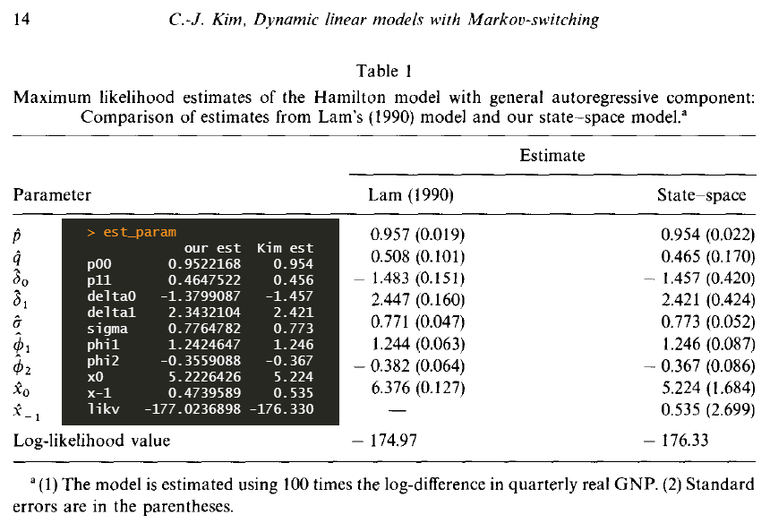
The following R code estimate parameters of example model in Kim (1994) with U.S. real GNP data ranging from 1952.4 to 1984.4.
The original gauss code can be found at Prof. Kim’s web site (http://econ.korea.ac.kr/~cjkim/SSMARKOV.htm) where you can find bunch of gauss programs for regime switching state space model and Gibbs sampling. In the following R code, I use the same variable name in most case for a comparison purpose.
#========================================================# # Quantitative ALM, Financial Econometrics & Derivatives # ML/DL using R, Python, Tensorflow by Sang-Heon Lee # # https://kiandlee.blogspot.com #——————————————————–# # Lam’s generalized Hamilton model in Kim (1994) #========================================================# graphics.off() # clear all graphs rm(list = ls()) # remove all files from your workspace #======================================= # Functions #======================================= # parameter constraints trans <– function(b0){ b1 <– b0 # probability b1[1:2] <– exp(b0[1:2])/(1+exp(b0[1:2])) # variance b1[5] <– b0[5]^2 # AR(1), AR(2) coefficients XX6 <– b0[6]/(1+abs(b0[6])) XX7 <– b0[7]/(1+abs(b0[7])) b1[6] <– XX6 + XX7 b1[7] <– –1*XX6*XX7 return(b1) } # Kim filter = Hamilton + Kalman loglike <– function(param_unc, y) { # param_unc = init_param_unc; y = y nobs <– length(y) param <– trans(param_unc) p11 <– param[1] # Pr[St=1/St-1=1] p00 <– param[2] # Pr[St=0/St-1=0] MU0 <– param[3] # delta0 MU1 <– MU0 + param[4] # delta0 + delta1 VAR_W <– param[5] # sigma^2 phi1 <– param[6] # AR(1) phi2 <– param[7] # AR(2) R <– matrix(0,1,1) Q <– rbind(c(VAR_W, 0), c(0, 0)) H <– t(c(1, –1)) F <– rbind(c(phi1, phi2), c(1, 0)) # initialization B_LL0 <– B_LL1 <– param[8:9] #c(0,0) P_LL1 <– P_LL0 <– matrix(solve(diag(4) – kronecker(F,F))%*% as.vector(Q), nrow = 2) # initialization with steady state probabilities PROB_1 <– (1–p00)/(2–p11–p00) #Pr[S_0=1/Y_0] PROB_0 <– 1–PROB_1 #Pr[S_0=0/Y_0] #—————————————— # START ITERATION #—————————————— likv <– 0.0 for(t in 1:nobs) { #——————————— # KALMAN FILTER #——————————— # state prediction B_TL00 <– F %*% B_LL0 # S=0, S’=0 B_TL01 <– F %*% B_LL0 # S=0, S’=1 B_TL10 <– F %*% B_LL1 # S=1, S’=0 B_TL11 <– F %*% B_LL1 # S=1, S’=1 # state prediction uncertainty P_TL00 <– F %*% P_LL0 %*% t(F) + Q P_TL01 <– F %*% P_LL0 %*% t(F) + Q P_TL10 <– F %*% P_LL1 %*% t(F) + Q P_TL11 <– F %*% P_LL1 %*% t(F) + Q # forecast fit00 <– H %*% B_TL00 + MU0 fit01 <– H %*% B_TL01 + MU1 fit10 <– H %*% B_TL10 + MU0 fit11 <– H %*% B_TL11 + MU1 # forecast error F_CAST00 <– y[t] – fit00 F_CAST01 <– y[t] – fit01 F_CAST10 <– y[t] – fit10 F_CAST11 <– y[t] – fit11 # forecast error variance SS00 <– H %*% P_TL00 %*% t(H) + R SS01 <– H %*% P_TL01 %*% t(H) + R SS10 <– H %*% P_TL10 %*% t(H) + R SS11 <– H %*% P_TL11 %*% t(H) + R # Kalman gain kg00 <– P_TL00 %*% t(H) %*% solve(SS00) kg01 <– P_TL01 %*% t(H) %*% solve(SS01) kg10 <– P_TL10 %*% t(H) %*% solve(SS10) kg11 <– P_TL11 %*% t(H) %*% solve(SS11) # updating B_TT00 <– B_TL00 + kg00 %*% F_CAST00 B_TT01 <– B_TL01 + kg01 %*% F_CAST01 B_TT10 <– B_TL10 + kg10 %*% F_CAST10 B_TT11 <– B_TL11 + kg11 %*% F_CAST11 P_TT00 <– (diag(2) – kg00 %*% H ) %*% P_TL00 P_TT01 <– (diag(2) – kg01 %*% H ) %*% P_TL01 P_TT10 <– (diag(2) – kg10 %*% H ) %*% P_TL10 P_TT11 <– (diag(2) – kg11 %*% H ) %*% P_TL11 #——————————— # HAMILTON FILTER #——————————— # Pr[St,Yt/Yt-1] NORM_PDF00 <– dnorm(F_CAST00,0,sqrt(SS00)) NORM_PDF01 <– dnorm(F_CAST01,0,sqrt(SS01)) NORM_PDF10 <– dnorm(F_CAST10,0,sqrt(SS10)) NORM_PDF11 <– dnorm(F_CAST11,0,sqrt(SS11)) PR_VL00 <– NORM_PDF00*( p00)*PROB_0 PR_VL01 <– NORM_PDF01*(1–p00)*PROB_0 PR_VL10 <– NORM_PDF10*(1–p11)*PROB_1 PR_VL11 <– NORM_PDF11*( p11)*PROB_1 # f(y_t|Y_{t-1}) PR_VAL <– PR_VL00 + PR_VL01 + PR_VL10 + PR_VL11 # Pr[St,St-1/Yt] PRO_00 <– as.numeric(PR_VL00/PR_VAL) PRO_01 <– as.numeric(PR_VL01/PR_VAL) PRO_10 <– as.numeric(PR_VL10/PR_VAL) PRO_11 <– as.numeric(PR_VL11/PR_VAL) # Pr[St/Yt] PROB_0 <– PRO_00 + PRO_10 PROB_1 <– PRO_01 + PRO_11 #——————————— # Kim’s Collapsing #——————————— B_LL0 <– (PRO_00*B_TT00 + PRO_10*B_TT10)/PROB_0 B_LL1 <– (PRO_01*B_TT01 + PRO_11*B_TT11)/PROB_1 temp00 <– (B_LL0–B_TT00) %*% t(B_LL0–B_TT00) temp10 <– (B_LL0–B_TT10) %*% t(B_LL0–B_TT10) temp01 <– (B_LL1–B_TT01) %*% t(B_LL1–B_TT01) temp11 <– (B_LL1–B_TT11) %*% t(B_LL1–B_TT11) P_LL0 <– (PRO_00*(P_TT00 + temp00) + PRO_10*(P_TT10 + temp10))/PROB_0 P_LL1 <– (PRO_01*(P_TT01 + temp01) + PRO_11*(P_TT11 + temp11))/PROB_1 likv = likv –log(PR_VAL) } return(likv) } #======================================= # Run #======================================= # Lam’s Real GNP Data Set : #1952.3 ~ 1984.4 rgnp <– c( 1378.2, 1406.8, 1431.4, 1444.9, 1438.2, 1426.6, 1406.8, 1401.2, 1418 , 1438.8, 1469.6, 1485.7, 1505.5, 1518.7, 1515.7, 1522.6, 1523.7, 1540.6, 1553.3, 1552.4, 1561.5, 1537.3, 1506.1, 1514.2, 1550 , 1586.7, 1606.4, 1637 , 1629.5, 1643.4, 1671.6, 1666.8, 1668.4, 1654.1, 1671.3, 1692.1, 1716.3, 1754.9, 1777.9, 1796.4, 1813.1, 1810.1, 1834.6, 1860 , 1892.5, 1906.1, 1948.7, 1965.4, 1985.2, 1993.7, 2036.9, 2066.4, 2099.3, 2147.6, 2190.1, 2195.8, 2218.3, 2229.2, 2241.8, 2255.2, 2287.7, 2300.6, 2327.3, 2366.9, 2385.3, 2383 , 2416.5, 2419.8, 2433.2, 2423.5, 2408.6, 2406.5, 2435.8, 2413.8, 2478.6, 2478.4, 2491.1, 2491 , 2545.6, 2595.1, 2622.1, 2671.3, 2734 , 2741 , 2738.3, 2762.8, 2747.4, 2755.2, 2719.3, 2695.4, 2642.7, 2669.6, 2714.9, 2752.7, 2804.4, 2816.9, 2828.6, 2856.8, 2896 , 2942.7, 3001.8, 2994.1, 3020.5, 3115.9, 3142.6, 3181.6, 3181.7, 3178.7, 3207.4, 3201.3, 3233.4, 3157 , 3159.1, 3199.2, 3261.1, 3250.2, 3264.6, 3219 , 3170.4, 3179.9, 3154.5, 3159.3, 3186.6, 3258.3, 3306.4, 3365.1, 3444.7, 3487.1, 3507.4, 3520.4) # # GNP growth rate : 1952.4 ~ 1984.4 y <– diff(log(rgnp),1)*100 # initial guess init_param_unc <– c(3.5,0.0,–0.4,1.7,0.5,1,0.7,1,1) # optimization mle <– optim(init_param_unc, loglike, method=c(“BFGS”), control=list(maxit=50000,trace=2), y=y) mle <– optim(mle$par, loglike, method=c(“Nelder-Mead”), control=list(maxit=50000,trace=2), y=y) # compare estimation results with Kim (1994) paper est_param <– cbind(c(trans(mle$par), –mle$value), c(0.954, 0.456, –1.457, 2.421, 0.773, 1.246, –0.367, 5.224, 0.535, –176.33)) est_param[5,1] <– sqrt(est_param[5,1]) # var -> std colnames(est_param) <– c(“our est”, “Kim est”) rownames(est_param) <– c(“p00”,“p11”,“delta0”, “delta1”, “sigma”, “phi1”, “phi2”,“x0”,“x-1”,“likv”) est_param | cs |
The following figure shows that our estimated parameters and evaluated log likelihood are very similar to results of Kim (1994).
Concluding Remarks
This post dealt with the regime switching state space model. It seems that this regime switching modeling approach is widely and actively used in trading practice. I tried to give intuitive and sequential explanations and to implement R code for the regime switching state space model by using Kim (1994) algorithm. For more information about this modeling techniques, I refer the reader to Kim and Nelson (1999). \(\blacksquare\)
Kim, Chang-Jin (1994) Dynamic Linear Models with Markov-switching, Journal of Econometrics 60-1, pp. 1-22.
Kim, C.-J. and C. R. Nelson (1999) State-Space Models with Regime Switching: Classical and Gibbs-Sampling Approaches with Applications. MIT Press. (http://econ.korea.ac.kr/~cjkim/SSMARKOV.htm)
To leave a comment for the author, please follow the link and comment on their blog: K & L Fintech Modeling.
R-bloggers.com offers daily e-mail updates about R news and tutorials about learning R and many other topics. Click here if you're looking to post or find an R/data-science job.
Want to share your content on R-bloggers? click here if you have a blog, or here if you don't.