
Kim (1994) Smoother Algorithm in Regime Switching Model using R code
[This article was first published on K & L Fintech Modeling, and kindly contributed to R-bloggers]. (You can report issue about the content on this page here)
Want to share your content on R-bloggers? click here if you have a blog, or here if you don't.
This post explains smoothing algorithm of a regime switching model, which is known as Kim (1994) smoother. It is known that smoothing algorithm is more difficult to understand than filtering algorithm. For this perspective, I give detailed derivations and use more simplified expressions with which I match variables in R code. Want to share your content on R-bloggers? click here if you have a blog, or here if you don't.
Kim’s Smoother Algorithm in Regime Switching Model
In the previous posts below, we used MSwM R package or implement a R code to estimate parameters of the two-state regime switching model. In this post we try to calculate backward smoothed probabilities by using Kim (1994) algorithm.
Regime Switching model
A two-state regime switching linear regression model and a transition probability matrix are of the following forms.
\[\begin{align} &y_t = c_{s_t} + \beta_{s_t}y_{t-1} + \epsilon_{s_t,t}, \quad \epsilon_{s_t,t} \sim N(0,\sigma_{s_t}) \\ \\ &P(s_t=j|s_{t−1}=i) = P_{ij} = \begin{bmatrix} p_{00} & p_{01} \\ p_{10} & p_{11} \end{bmatrix} \end{align}\] Here \(s_t\) can take on 0 or 1 and \(p_{ij}\) is the probability of transitioning from regime \(i\) at time \(t-1\) to regime \(j\) at time \(t\).
Derivation of Kim (1994) Smoothing Algorithm
Kim (1994) Smoother is used following a run of Hamilton filtering using all the information in the sample. Smoothing algorithm starts at T and is run from T-1 to 1. Similar to the filtered probability, the smoothed probability can be formulated in the following way except the information set (\( \tilde{y}_T = \{y_1, y_2,…, y_{T-1}, y_T\}\)).
\[\begin{align} P(s_t = j|\tilde{y}_T;\mathbf{\theta}) \\ \end{align}\]
if we abstract from \(\mathbf{\theta}\) for simplicity. \(P(s_t = j|\tilde{y}_T)\) can be decomposed into
\[\begin{align} P(s_t = j|\tilde{y}_T) &= P(s_t = j, s_{t+1} = 0 | \tilde{y}_T) \\ &+ P(s_t = j, s_{t+1} = 1 | \tilde{y}_T) \end{align}\]
Therefore we need to derive the expression for \(P(s_t = j, s_{t+1} = k | \tilde{y}_T) \). This can be derived by using the Bayes theorem.
\[\begin{align} &P(s_t = j,s_{t+1} = k | \tilde{y}_T) \\ & = P(s_{t+1} = k|\tilde{y}_T) \times P(s_t = j|s_{t+1} = k, \tilde{y}_T) \\ & = P(s_{t+1} = k|\tilde{y}_T) \times P(s_t = j|s_{t+1} = k, \color{red}{\tilde{y}_t}) \end{align}\]
Reducing information set \(\tilde{y}_T \rightarrow \color{red}{\tilde{y}_t} \) in the right second term is possible due to the AR(1) model. Since \(s_{t+1}\) is known and fixed as \(k\), more than \(\tilde{y}_{t}\) contain no information about \(s_t\). In other words, conditioning \(s_{t+1} = k\) cuts information after time \(t\). Remaining derivation carries on.
\[\begin{align} &P(s_t = j,s_{t+1} = k | \tilde{y}_T) \\ & =(s_{t+1} = k|\tilde{y}_T) \times \color{red}{P(s_t = j|s_{t+1} = k, \tilde{y}_t)} \\ & =P(s_{t+1} = k|\tilde{y}_T) \times \color{red}{\frac{ P(s_t = j,s_{t+1} = k | \tilde{y}_t)} {P(s_{t+1} = k | \tilde{y}_t)}}\\ & = \frac{P(s_{t+1} = k|\tilde{y}_T) \times \color{green }{P(s_t = j| \tilde{y}_t) \times P(s_{t+1} = k| s_t = j)}} {P(s_{t+1} = k | \tilde{y}_t)} \\ &= \color{blue}{\frac{SP_{t+1}^k \times fp_t^j \times p^{jk}} {ps_{t+1,t}^k}} \end{align}\]
The last expression is of heuristic notations which I make for an easy understanding. Using the following heuristic notations, we can easily relate this derivation to the implementation of R code.
\[\begin{align} \color{blue}{SP_t^k} &= \text{smoothing probability for k-state at time t} \\ \color{blue}{fp_t^j } &= \text{filtered probability for j-state at time t} \\ \color{blue}{p^{jk} } &= \text{transition probability from j to k} \\ \color{blue}{ps_{t+1,t}^k} &= \text{t+1 predicted state for k-state at time t} \end{align}\]
Now we can calculate \(P(s_t = j|\tilde{y}_T) \) with \(P(s_t = j,s_{t+1} = k | \tilde{y}_T)\).
\[\begin{align} &P(s_t = j|\tilde{y}_T) \\ &= P(s_t = j, s_{t+1} = 0 | \tilde{y}_T) + P(s_t = j, s_{t+1} = 1 | \tilde{y}_T) \\ &= \frac{P(s_{t+1} = 0 |\tilde{y}_T) \times P(s_t = j| \tilde{y}_t) \times P(s_{t+1} = 0| s_t = j)} {P(s_{t+1} = 0 | \tilde{y}_t)} \\ &+\frac{P(s_{t+1} = 1|\tilde{y}_T) \times P(s_t = j| \tilde{y}_t) \times P(s_{t+1} = 1| s_t = j)} {P(s_{t+1} = 1 | \tilde{y}_t)} \end{align}\]
Kim (1994) Smoother Equation for Two-state model
In standard notation, we can find the recursive structure of backward smoothing probabilities (\(P(s_t = j|\tilde{y}_T), j=0,1\)).
| \[\begin{align} &\color{blue}{P(s_t = 0|\tilde{y}_T)} \\ &= \frac{\color{blue}{P(s_{t+1} = 0 |\tilde{y}_T)} \times P(s_t = 0| \tilde{y}_t) \times P(s_{t+1} = 0| s_t = 0)} {P(s_{t+1} = 0 | \tilde{y}_t)} \\ &+\frac{\color{red}{P(s_{t+1} = 1|\tilde{y}_T)} \times P(s_t = 0| \tilde{y}_t) \times P(s_{t+1} = 1| s_t = 0)} {P(s_{t+1} = 1 | \tilde{y}_t)} \\\\ &\color{red}{P(s_t = 1|\tilde{y}_T)} \\ &= \frac{\color{blue}{P(s_{t+1} = 0 |\tilde{y}_T)} \times P(s_t = 1| \tilde{y}_t) \times P(s_{t+1} = 0| s_t = 1)} {P(s_{t+1} = 0 | \tilde{y}_t)} \\ &+\frac{\color{red}{P(s_{t+1} = 1|\tilde{y}_T)} \times P(s_t = 1| \tilde{y}_t) \times P(s_{t+1} = 1| s_t = 1)} {P(s_{t+1} = 1 | \tilde{y}_t)} \end{align}\] |
In my heuristic notation, we can also find the recursive structure of backward smoothing probabilities (\(SP_t^j, j=0,1\)).
\[\begin{align} &\color{blue}{SP_t^0} = \frac{\color{blue}{ps_{t+1}^0} \times fp_t^0 \times p^{00}} {ps_{t+1,t}^0} + \frac{\color{red}{SP_{t+1}^1} \times fp_t^0 \times p^{01}} {ps_{t+1,t}^1} \\\\ &\color{red}{SP_t^1} = \frac{\color{blue}{SP_{t+1}^0} \times fp_t^1 \times p^{10}} {ps_{t+1,t}^0} + \frac{\color{red}{SP_{t+1}^1} \times fp_t^1 \times p^{11}} {ps_{t+1,t}^1} \end{align}\] Here, we need to decompose t+1 state prediction at time t (\(ps_{t+1,t}^j \)), which is calculated from two components in the following way.
\[\begin{align} ps_{t+1,t}^j &= P(s_{t+1} = j | \tilde{y}_t) \\ &= P(s_{t+1} = j, s_{t} = 0 | \tilde{y}_t) + P(s_{t+1} = j, s_{t} = 1 | \tilde{y}_t) \\ &= P(s_{t} = 0 | \tilde{y}_t) \times P(s_{t+1} = j, s_{t} = 0) \\ &+ P(s_{t} = 1 | \tilde{y}_t) \times P(s_{t+1} = j, s_{t} = 1) \\ &= fp_t^0 \times p^{0j} + fp_t^1 \times p^{1j} \end{align}\]
At last, we can get the final heuristic expressions for Kim (1994) smoother as follows.
| \[\begin{align} &\color{blue}{SP_t^0} = \frac{\color{blue}{SP_{t+1}^0} \times fp_t^0 \times p^{00}} {fp_t^0 \times p^{00} + fp_t^1 \times p^{10} } + \frac{\color{red}{SP_{t+1}^1} \times fp_t^0 \times p^{01}} {fp_t^0 \times p^{01} + fp_t^1 \times p^{11} } \\\\ &\color{red}{SP_t^1} = \frac{\color{blue}{SP_{t+1}^0} \times fp_t^1 \times p^{10}} {fp_t^0 \times p^{00} + fp_t^1 \times p^{10} } + \frac{\color{red}{SP_{t+1}^1} \times fp_t^1 \times p^{11}} {fp_t^0 \times p^{01} + fp_t^1 \times p^{11} } \end{align}\] |
As we will see later, the above simplified expressions can be implemented as the following R code snippet through the one-to-one mappings.
# S(t)=0, S(t+1)=0 p1 <– (sp[t+1,1]*fp[t,1]*p00)/ (fp[t,1]*p00 + fp[t,2]*p10) # S(t)=0, S(t+1)=1 p2 <– (sp[t+1,2]*fp[t,1]*p01)/ (fp[t,1]*p01 + fp[t,2]*p11) # S(t)=1, S(t+1)=0 p3 <– (sp[t+1,1]*fp[t,2]*p10)/ (fp[t,1]*p00 + fp[t,2]*p10) # S(t)=1, S(t+1)=1 p4 <– (sp[t+1,2]*fp[t,2]*p11)/ (fp[t,1]*p01 + fp[t,2]*p11) sp[t,1] <– p1+p2 sp[t,2] <– p3+p4 | cs |
R code
The following R code calculates backward smoothing probabilities of the two-state regime switching model with the same data (12M year on year U.S. CPI inflation rate) as in the previous post.
Before this R code is run, R code for Hamilton filtering in the previous post must be run since redundant codes are not included in the following R code.
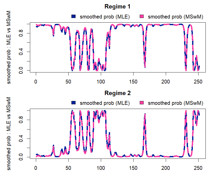
The following results show that smoothed probabilities are more smoother than filtered probabilities as expected.

From the figure below we can easily find that smoothed probabilities from MSwM R package and our estimates are almost the same except some earlier periods.
In this post, we learn Kim (1994) smoother algorithm in regime switching model more deeply, implement R code, and compare our results with that of MSwM R package. Since smoothed probabilities use all the information in sample, it shows more smooth behavior. \(\blacksquare\)
Chang-Jin Kim (1994) Dynamic Linear Models with Markov-switching, Journal of Econometrics 60-1, pp. 1-22.
#========================================================# # Quantitative ALM, Financial Econometrics & Derivatives # ML/DL using R, Python, Tensorflow by Sang-Heon Lee # # https://kiandlee.blogspot.com #——————————————————–# # Hamilton Regime Switching Model – Kim (1994) smoother #========================================================# ########################################################## ## At first, Run R code for Hamilton Filtering # in the following post # # https://kiandlee.blogspot.com/2022/02/ # hamilton-regime-switching-model-using-r.html # ########################################################## #——————————————————– # Smoother function for regime switching AR(1) model #——————————————————– kim.smoother <– function(param,x,y){ # param = mle$par; x = y1; y = y0 nobs = length(y) # constant, AR(1), sigma const0 <– param[1]; const1 <– param[2] beta0 <– param[3]; beta1 <– param[4] sigma0 <– param[5]; sigma1 <– param[6] p00 <– 1/(1+exp(–param[7])) p11 <– 1/(1+exp(–param[8])) p01 <– 1–p00; p10 <– 1–p11 # previous and updated state (fp) ps_i0 <– us_j0 <– ps_i1 <– us_j1 <– NULL # steady state probability sspr1 <– (1–p00)/(2–p11–p00) sspr0 <– 1–sspr1 # initial values for states (fp0) us_j0 <– sspr0 us_j1 <– sspr1 # filtered and smoothed probability fp <– sp <– matrix(0,nrow = length(y),ncol = 2) # run Hamilton filter and get filtered estimates hf <– hamilton.filter(param, x = x, y = y) # get filtered outputs fp <– hf$fp; # filtered probability ps <– hf$ps; # predicted state T <– nobs sp <– data.frame(s0=rep(0,T),s1=rep(0,T)) # at T, filtered and smoothed prob are same sp[T,] <– fp[T,] # iteration from T-1 to 1 for(is in (T–1):1){ # S(t)=0, S(t+1)=0 p1 <– (sp[is+1,1]*fp[is,1]*p00)/ (fp[is,1]*p00 + fp[is,2]*p10) # S(t)=0, S(t+1)=1 p2 <– (sp[is+1,2]*fp[is,1]*p01)/ (fp[is,1]*p01 + fp[is,2]*p11) # S(t)=1, S(t+1)=0 p3 <– (sp[is+1,1]*fp[is,2]*p10)/ (fp[is,1]*p00 + fp[is,2]*p10) # S(t)=1, S(t+1)=1 p4 <– (sp[is+1,2]*fp[is,2]*p11)/ (fp[is,1]*p01 + fp[is,2]*p11) sp[is,1] <– p1+p2; sp[is,2] <– p3+p4 } return(sp) } # run smoother sp <– kim.smoother(mle$par,x = y1, y = y0) # draw some graphs for comparisons br <– “bottomright” x11(); par(mfrow=c(2,1)) vcol <– c(“green”,“blue”) ylab <– “filtered & smoothed prob” vleg <– c(“filtered prob”,“smoothed prob”) matplot(cbind(hf$fp[,1],sp[,1]), main = “Regime 1”, type=“l”, col = vcol, lwd = 3, lty = 1, ylab = ylab) legend(br, legend = vleg, fill = vcol, inset=c(0,1), xpd=TRUE, horiz=TRUE, bty=“n”) matplot(cbind(hf$fp[,2],sp[,2]), main = “Regime 2”, type=“l”, col = vcol, lwd = 3, lty = 1, ylab = ylab) legend(br, legend = vleg, fill = vcol, inset=c(0,1), xpd=TRUE, horiz=TRUE, bty=“n”) x11(); par(mfrow=c(2,1)) vcol <– c(“#00239CFF”,“#FF3EA5FF”) ylab <– “smoothed prob : MLE vs MSwM” vleg <– c(“smoothed prob (MLE)”,“smoothed prob (MSwM)”) matplot(cbind(sp[,1], rsm@Fit@smoProb[–1,2]), type=“l”, main = “Regime 1”, col = vcol, lwd = 4,ylab = ylab) legend(br, legend = vleg, fill = vcol, inset=c(0,1), xpd=TRUE, horiz=TRUE, bty=“n”) matplot(cbind(sp[,2], rsm@Fit@smoProb[–1,1]), type=“l”, main = “Regime 2”, col = vcol, lwd = 4,ylab = ylab) legend(br, legend = vleg, fill = vcol, inset=c(0,1), xpd=TRUE, horiz=TRUE, bty=“n”) | cs |
The following results show that smoothed probabilities are more smoother than filtered probabilities as expected.
From the figure below we can easily find that smoothed probabilities from MSwM R package and our estimates are almost the same except some earlier periods.
Concluding Remarks
In this post, we learn Kim (1994) smoother algorithm in regime switching model more deeply, implement R code, and compare our results with that of MSwM R package. Since smoothed probabilities use all the information in sample, it shows more smooth behavior. \(\blacksquare\)
Chang-Jin Kim (1994) Dynamic Linear Models with Markov-switching, Journal of Econometrics 60-1, pp. 1-22.
To leave a comment for the author, please follow the link and comment on their blog: K & L Fintech Modeling.
R-bloggers.com offers daily e-mail updates about R news and tutorials about learning R and many other topics. Click here if you're looking to post or find an R/data-science job.
Want to share your content on R-bloggers? click here if you have a blog, or here if you don't.