
Hamilton Regime Switching Model using R code
[This article was first published on K & L Fintech Modeling, and kindly contributed to R-bloggers]. (You can report issue about the content on this page here)
Want to share your content on R-bloggers? click here if you have a blog, or here if you don't.
This post estimates parameters of a regime switching model directly by using R code. The same model was already implemented by using MSwM R package in the previous post. Through this hand-on example I hope we can learn the process of Hamilton filtering more deeply. Want to share your content on R-bloggers? click here if you have a blog, or here if you don't.
Hamilton Regime Switching Model using R code
In the previous post below, we used MSwM R package to estimate parameters of the two-state regime switching model. In this post we directly estimate it with the sequence of Hamilton filter.
Regime Switching model
A two-state regime switching linear regression model and a transition probability matrix are of the following forms.
\[\begin{align} &y_t = c_{s_t} + \beta_{s_t}x_t + \epsilon_{s_t,t}, \quad \epsilon_{s_t,t} \sim N(0,\sigma_{s_t}) \\ \\ &P(s_t=j|s_{t−1}=i) = P_{ij} = \begin{bmatrix} p_{00} & p_{01} \\ p_{10} & p_{11} \end{bmatrix} \end{align}\] Here \(s_t\) can take on 0 or 1 and \(p_{ij}\) is the probability of transitioning from regime \(i\) at time \(t-1\) to regime \(j\) at time \(t\).
Hamilton Filtering
Hamilton filter is of the following sequence as we presented it in the previous post.
| 1) \(t-1\) state (previous state) \[\begin{align} \xi_{i,t-1} &= P(s_{t-1} = i|\tilde{y}_{t-1};\mathbf{\theta}) \end{align}\] 2) state transition from \(i\) to \(j\) (state propagation) \[\begin{align} p_{ij} \end{align}\] 3) densities under the two regimes at \(t\) (data observations and state dependent errors) \[\begin{align} \eta_{jt} = \frac{1}{\sqrt{2\pi}\sigma}\exp\left[-\frac{(y_t-c_j-\beta_j x_t)^2}{2\sigma_j^2}\right] \end{align}\] 4) conditional density of the time \(t\) observation (combined likelihood with state being collapsed): \[\begin{align} f(y_t|\tilde{y}_{t-1};\mathbf{\theta}) &= \xi_{0,t-1}p_{00}\eta_{0t} + \xi_{0,t-1}p_{01}\eta_{1t} \\ &+ \xi_{1,t-1}p_{10}\eta_{0t} + \xi_{1,t-1}p_{11}\eta_{1t} \end{align}\] 5) \(t\) posterior state (corrected from previous state) \[\begin{align} \xi_{jt} = \frac{\sum_{i=0}^{1} \xi_{i,t-1}p_{ij}\eta_{jt}} {f(y_t|\tilde{y}_{t-1};\mathbf{\theta})} \end{align}\] 6) use posterior state at time \(t\) as previous state a time \(t+1\) (substitution) \[\begin{align} \xi_{jt} \rightarrow \xi_{i,t-1} \end{align}\] 7) iterate 1) ~ 6) from t = 1 to T |
As a result of executing this iteration, the sample conditional log likelihood of the observed data can be calculated in the following way. \[\begin{align} \log f(\tilde{y}_{t}|y_0;\mathbf{\theta}) = \sum_{t=1}^{T}{ f(y_t|\tilde{y}_{t-1};\mathbf{\theta}) } \end{align}\] With this log-likelihood function, we use a numerical optimization to find the best fitting parameter set(\(\tilde{\mathbf{\theta}}\)).
Numerical Optimization
To start iterations of the Hamilton filter, we need to set \(\xi_{i,0} \) and in most cases the unconditional state probabilities are used. \[\begin{align} \xi_{0,0} &= \frac{1 – p_{11}}{2 – p_{00} – p_{11}} \\ \xi_{1,0} &= 1 – \xi_{0,0} \end{align}\]
R code
The following R code implement MLE parameter estimation of two-state regime switching model with the same date as in the previous post. This code is line with the process of the Hamilton filtering.
#========================================================# # Quantitative ALM, Financial Econometrics & Derivatives # ML/DL using R, Python, Tensorflow by Sang-Heon Lee # # https://kiandlee.blogspot.com #——————————————————–# # Hamilton Regime Switching Model – AR(1) inflation model #========================================================# graphics.off() # clear all graphs rm(list = ls()) # remove all files from your workspace library(MSwM) #—————————————— # Data : U.S. CPI inflation 12M, yoy #—————————————— inf <– c( 3.6536,3.4686,2.9388,3.1676,3.5011,3.144,2.6851,2.6851,2.5591, 2.1053,1.8767,1.5909,1.1888,1.13,1.3537,1.6306,1.2332,1.0635, 1.455,1.7324,1.5046,2.0068,2.2285,2.45,2.7201,3.0976,2.9804, 2.1518,1.8764,1.93,2.0347,2.1919,2.3505,2.0214,1.91,2.0148, 2.006,1.6744,1.7251,2.2667,2.8566,3.1185,2.8972,2.5155,2.5075, 3.1411,3.5576,3.2877,2.8052,3.0073,3.1565,3.3065,2.8289,2.5093, 3.0211,3.582,4.6328,4.2581,3.284,3.284,3.9401,3.5736,3.3608, 3.5501,3.9002,4.0967,4.0227,3.8514,1.9921,1.3965,1.9496,2.4927, 2.0545,2.3914,2.7598,2.5599,2.6738,2.6571,2.2914,1.8797,2.7944, 3.547,4.2803,4.0266,4.205,4.0594,3.8979,3.8295,4.007,4.818, 5.3517,5.1719,4.8345,3.6631,1.0939,–0.0222,–0.1137,0.0085,–0.4475, –0.578,–1.021,–1.2368,–1.9782,–1.495,–1.3875,–0.2242,1.8965,2.7753, 2.5873,2.1285,2.2604,2.1828,1.9837,1.1153,1.3319,1.1436,1.1121, 1.1599,1.0787,1.4276,1.6865,2.1026,2.5855,3.0308,3.4005,3.4424, 3.5173,3.6862,3.7417,3.4617,3.3932,3.0161,2.9644,2.857,2.5501, 2.2477,1.723,1.6403,1.4076,1.6719,1.931,2.1328,1.7801,1.7442, 1.67,1.998,1.5073,1.1324,1.3808,1.7012,1.8679,1.5271,1.0888, 0.873,1.2253,1.5015,1.5458,1.1142,1.5998,1.9951,2.1438,2.0381, 1.955,1.7006,1.67,1.5967,1.224,0.651,–0.2302,–0.0871,–0.022, –0.1041,0.035,0.1794,0.2254,0.241,0.0088,0.1275,0.4354,0.6367, 1.2299,0.8437,0.8877,1.1658,1.0727,1.0735,0.8646,1.0498,1.5368, 1.6719,1.6703,2.0301,2.4802,2.7167,2.3602,2.186,1.866,1.6498, 1.7255,1.9187,2.2042,2.0132,2.1872,2.0797,2.0722,2.2013,2.3318, 2.427,2.7149,2.7997,2.8511,2.6282,2.2586,2.4991,2.1768,1.902, 1.4846,1.461,1.8386,1.9981,1.8117,1.6863,1.8058,1.7261,1.7098, 1.7591,2.0231,2.2363,2.4441,2.2881,1.5004,0.3386,0.2233,0.7252, 1.0414,1.3161,1.4001,1.1876,1.1324,1.2918,1.3607,1.6618,2.6031, 4.0692,4.809,5.1876,5.1478,5.0717,5.2377,6.0564,6.6541,6.8811) ninf <– length(inf) # y and its first lag y0 <– inf[2:ninf]; y1 <– inf[1:(ninf–1)] df <– data.frame(y = y0, y1 = y1) #—————————————— # Single State : OLS #—————————————— lrm <– lm(y~y1,df) #—————————————— # Two State : Markov Switching (MSwM) #—————————————— k <– 2 # two-regime mv <– 3 # means of 2 variables + 1 for volatility rsm=msmFit(lrm, k=2, p=0, sw=rep(TRUE, mv), control=list(parallel=FALSE)) #—————————————— # function : Hamilton filter #—————————————— # y = const0 + beta0*x + e0, # y = const1 + beta1*x + e1, # # e0 ~ N(0,sigma0) : regime 1 # e1 ~ N(0,sigma1) : regime 2 ##—————————————— hamilton.filter <– function(param,x,y){ # param = mle$par; x = y1; y = y0 nobs = length(y) # constant, AR(1), sigma const0 <– param[1]; const1 <– param[2] beta0 <– param[3]; beta1 <– param[4] sigma0 <– param[5]; sigma1 <– param[6] # restrictions on range of probability (0~1) p00 <– 1/(1+exp(–param[7])) p11 <– 1/(1+exp(–param[8])) p01 <– 1–p00; p10 <– 1–p11 # previous and updated state (fp) ps_i0 <– us_j0 <– ps_i1 <– us_j1 <– NULL # steady state probability sspr1 <– (1–p00)/(2–p11–p00) sspr0 <– 1–sspr1 # initial values for states (fp0) us_j0 <– sspr0 us_j1 <– sspr1 # predicted state, filtered and smoothed probability ps <– fp <– sp <– matrix(0,nrow = length(y),ncol = 2) loglike <– 0 for(t in 1:nobs){ #) t-1 state (previous state) # -> use previous updated state ps_i0 <– us_j0 ps_i1 <– us_j1 # 2) state transition from i to j (state propagation) # -> use time invariant transition matrix # 3) densities under the two regimes at t # (data observations and state dependent errors) # regression error er0 <– y[t] – const0 – beta0*x[t] er1 <– y[t] – const1 – beta1*x[t] eta_j0 <– (1/(sqrt(2*pi*sigma0^2)))*exp(–(er0^2)/(2*(sigma0^2))) eta_j1 <– (1/(sqrt(2*pi*sigma1^2)))*exp(–(er1^2)/(2*(sigma1^2))) #4) conditional density of the time t observation # (combined likelihood with state being collapsed): f_yt <– ps_i0*p00*eta_j0 + # 0 -> 0 ps_i0*p01*eta_j1 + # 0 -> 1 ps_i1*p10*eta_j0 + # 1 -> 0 ps_i1*p11*eta_j1 # 1 -> 1 # check for numerical instability if( f_yt < 0 || is.na(f_yt)) { loglike <– –100000000; break } # 5) updated states us_j0 <– (ps_i0*p00*eta_j0+ps_i1*p10*eta_j0)/f_yt us_j1 <– (ps_i0*p01*eta_j1+ps_i1*p11*eta_j1)/f_yt ps[t,] <– c(ps_i0, ps_i0) # predicted states fp[t,] <– c(us_j0, us_j1) # filtered probability loglike <– loglike + log(f_yt) } return(list(loglike = –loglike, fp = fp, ps = ps )) } # objective function for optimization rs.est <– function(param,x,y){ return(hamilton.filter(param,x,y)$loglike) } #—————————————— # Run numerical optimization for estimation #—————————————— # use linear regression estimates as initial guesses init_guess <– c(lrm$coefficients[1], lrm$coefficients[1], lrm$coefficients[2], lrm$coefficients[2], summary(lrm)$sigma, summary(lrm)$sigma, 3, 2.9) # multiple optimization to reassess convergence mle <– optim(init_guess, rs.est, control = list(maxit=50000, trace=2), method=c(“BFGS”), x = y1, y = y0) mle <– optim(mle$par, rs.est, control = list(maxit=50000, trace=2), method=c(“Nelder-Mead”), x = y1, y = y0) #—————————————— # Report outputs #—————————————— # get filtering output : fp, ps hf <– hamilton.filter(mle$par,x = y1, y = y0) # draw filtered probabilities of two states x11(); par(mfrow=c(2,1)) matplot(cbind(rsm@Fit@filtProb[,1],hf$fp[,2]), main = “Regime 1”, type=“l”, cex.main=1) matplot(cbind(rsm@Fit@filtProb[,2],hf$fp[,1]), main = “Regime 2”, type=“l”, cex.main=1) # comparison of parameters invisible(print(“—–Comparison of two results—–“)) invisible(print(“constant and beta1”)) cbind(rsm@Coef, cbind(mle$par[1:2],mle$par[3:4])) invisible(print(“sigma”)) cbind(rsm@std, mle$par[5:6]) invisible(print(“p00, 011”)) cbind(diag(rsm@transMat), 1/(1+exp(–mle$par[7:8]))) invisible(print(“loglikelihood”)) cbind(rsm@Fit@logLikel, mle$value) | cs |
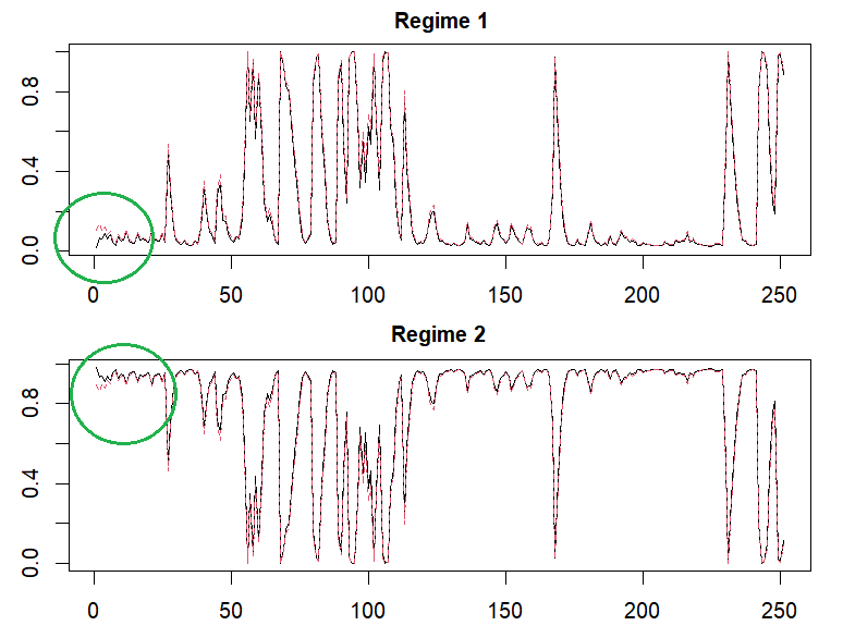
The following results show that two set of estimated parameters are slightly different but filtered probabilities are very similar. I think that some specifications including initial guess or initial probabilities results in this difference. Generally speaking, regime switching model is not easy to estimate since it is vulnerable to initial guesses. Therefore it is necessary to try to apply multiple initial guesses.

Now we can find that two-regime probabilities by using plotProb() function in MSwM R package and our estimate are similar except earlier period (green circle). I think that this difference is come from the difference of initial probabilities.
Concluding Remarks
In this post, we explains Hamilton regime switching model by taking AR(1) model as an example and implement R code without the help of MSwM R package. Smoothed probabilities as well as filtered probabilities are important since it use all information. In the next post, we will implement smoothed probabilities with some detail derivations. \(\blacksquare\)
To leave a comment for the author, please follow the link and comment on their blog: K & L Fintech Modeling.
R-bloggers.com offers daily e-mail updates about R news and tutorials about learning R and many other topics. Click here if you're looking to post or find an R/data-science job.
Want to share your content on R-bloggers? click here if you have a blog, or here if you don't.