Uncovered Interest Rate Parity and F-test on Regression Parameters using R
[This article was first published on K & L Fintech Modeling, and kindly contributed to R-bloggers]. (You can report issue about the content on this page here)
Want to share your content on R-bloggers? click here if you have a blog, or here if you don't.
This post explains how to perform the F-test of joint parameter restrictions on a linear regression model. As an example, we use the data in Chen and Tsang (2013), who introduce so called relative Nelson-Siegel factor model to predict exchange rates. We test whether data support uncovered interest rate parity (UIP) restrictions. Want to share your content on R-bloggers? click here if you have a blog, or here if you don't.
Uncovered Interest Rate Parity and Parameter Restriction
F-test of joint restrictions on coefficients
From an unrestricted linear regression, testing for joint linear restrictions on coefficients is carried out by using F, Wald, or likelihood ratio test. Among these test statistics, F-test statistic is widely used for this type of joint tests and has the following expression.
|
The meaning of F-test is intuitive. When parameter restrictions are statistically significant, the restricted model will not be much different from the unrestricted model. This results in the similar magnitude between residual sum of squares of two models.
Since a residual sum of squares is kind of a variance, its ratio follows F distribution as an introductory statistics textbook shows. Therefore, when parameter restrictions are important, F-statistic can not reject the null hypothesis of \(R \beta_U = b\), which indicates parameter restriction is supported.
Just so you know, the RLS estimator can be obtained from setting up a Lagrangian.
| \[\begin{align} \hat{\beta_R} = \hat{\beta_U} – (X’X)^{-1}R'(R(X’X)^{-1}R’)^{-1}(R\hat{\beta_U}-b) \end{align}\] |
Here, \(\hat{\beta_U}\) and \(\hat{\beta_R}\) denote OLS and RLS \(\beta\) estimates respectively.
Foreign Bond Return and Uncovered Interest Parity
From a risk-neutral investor, a domestic return of a foreign bond is the sum of 1) a foreign return of a foreign bond and 2) a domestic return of a foreign currency.
At maturity, 1) is converted into the domestic currency and 2) is realized so that if a foreign currency is stronger than a domestic currency, we can obtain additional FX return and vice versa. While a bond returns (held to maturity) is fixed at maturity, an exchange rate at maturity is uncertain. This leads to the importance of an expectation of FX rate. This kind of story is formally described in the form of the uncovered interest parity (UIP).
When F = foreign country and D = domestic (home) country are assumed and exchange rate is measured as the domestic currency price per unit of the foreign currency(\(=s:=s(D/F)\)), UIP condition has the following statement.
|
The UIP condition in Eq. (1) predicts the positive relationship between \(i^D_m – i^F_m\) and \(E_0 \Delta s_m\). In other words, a country with a higher interest tends to have its currency depreciation. In (2), risk-averse investors require additional risk premium for holding a foreign currency (3) : domestic return of a foreign bond – domestic return of a domestic bond > 0. Taking this additional risk premium into consideration, UIP condition is modified like (4).
Example : Chen and Tsang (2013) Relative NS model
The reason why I gave an introduction to the UIP condition is that some interesting hypothesis testing on linear restrictions is carried out in Chen and Tsang (2013) with the content of UIP condition.
Chen and Tsang (2013) introduce the relative Nelson-Siegel (NS) factor model for predicting exchange rate movements. They show that expected dynamics of future economic activity and the currency risk premiums are driven by relative NS factors which have differential expectations about two countries’ future output and inflation. And they also explain the UIP puzzle successfully and resolve it.
As an example for F-test, I borrow the following content from Chen and Tsang (2013), in which parameter restrictions on the relative NS factor model is carried out.
|
Since interest rate differential, \(i^D_{t,m} – i^F_{t,m}\) are decomposed into level, slope, and curvature factors, UIP regression can be represented by using the relative NS factor model. In other words, the relative NS factor model encompasses the UIP regression. The former is a unrestricted model and the latter a restricted model.
Now we test the following two linear restrictions on estimated parameters of the unrestricted relative NS factor model using F-test.
\[\begin{align} \frac{\beta_{2,m}}{\beta_{1,m}} &= \frac{1-\exp(-\lambda m)}{\lambda m} \\ \frac{\beta_{3,m}}{\beta_{1,m}} &= \frac{1-\exp(-\lambda m)}{\lambda m} – \exp(-\lambda m) \end{align}\]
Data
Chen and Tsang (2013) kindly provides their research data in their web site, from which I made a excel file to select some necessary data for our exercise. You can download this data at the K&L blog data page which is linked in K&L blog menu bar. Relative factors and log exchange rate are illustrated by the following figures.
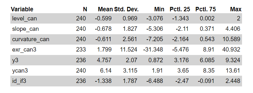
Data has the following descriptive statistics.
Here, level_can, slope_can, and curvature_can are relative level, slope, and curvature factors respectively (domestic factor(US) – foreign factor). exr_can3 is 3-month changes of exchange rate (USD/CAD). y3 and ycan3 are 3-month yields for the U.S and Canada and id_if3 is the interest rate differential.
R code
The following R code read input data regarding relative factors, 3M exchange rate changes, and so on and estimate the unrestricted relative NS factor regression model.
#========================================================# # Quantitative ALM, Financial Econometrics & Derivatives # ML/DL using R, Python, Tensorflow by Sang-Heon Lee # # https://kiandlee.blogspot.com #——————————————————–# # F-Test of restrictions on regression coefficients #========================================================# graphics.off() # clear all graphs rm(list = ls()) # remove all files from your workspace library(readxl) library(car) # linearHypothesis() setwd(“D:/SHLEE/blog/econometrics/linear_restrictions”) #——————————————- # data #——————————————- lambda = 0.0609; tau = 3 # month # read excel spot data file <– “CT_data_yield_fx.xlsx”; sheet <– “CT” df.data <– read_excel(file,sheet,col_names=TRUE) # interest rate differentials df.data$id_if3 <– df.data$y3 – df.data$ycan3 head(df.data) #——————————————- # Unrestricted Linear Regression #——————————————- # relative factor regression reg.U <– lm( exr_can3 ~ level_can + slope_can + curvature_can, data = df.data, na.action = na.omit) | cs |
In the subsequent R code, as an exercise for understanding F-test, we perform simple joint hypothesis testing on \(\beta_1 = \beta_2 = \beta_3 = 0\).
#———————————————– # F test by using linearHypothesis() #———————————————– # H0 : b1 = b2 = b3 = 0 #———————————————– H0 <– c(“level_can=0”,“slope_can=0”, “curvature_can=0”) # F test for coefficients restrictions linearHypothesis(reg.U, H0) #———————————————– # F test by mannual calculation #———————————————– # H0 : b1 = b2 = b3 = 0 #———————————————– # restricted regression model reg.R <– lm(exr_can3 ~ 1, data = df.data, na.action = na.omit) # input variables for F-test T <– length(reg.U$residuals) # # of observations K <– length(reg.U$coefficients) # # of parameters J <– 3 # # of restrictions # residual sum of squares RSSU <– sum(reg.U$residuals^2) RSSR <– sum(reg.R$residuals^2) # calculated F-test statistic F_test <– ((RSSR – RSSU)/J)/(RSSU/(T–K)) # 95% critical value and p-value qf(.95, df1=J, df2=(T–K)) # 95% critical value 1 – pf(F_test, df1=J, df2=(T–K)) # p-value | cs |
From the next results, the F-test indicate rejections of the zero restrictions as expected. We can also find that linearHypothesis() function and the manual calculation produce the same result.
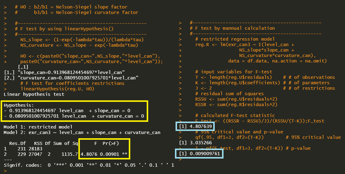
In the next R code, we perform F-test on restrictions on relative NS factor model which are explained the above section.
#———————————————– # F test by using linearHypothesis() #———————————————– # H0 : b2/b1 = Nelson-Siegel slope factor # b3/b1 = Nelson-Siegel curvature factor #———————————————– NS_slope <– (1–exp(–lambda*tau))/(lambda*tau) NS_curvature <– NS_slope – exp(–lambda*tau) H0 <– c(paste0(“slope_can=”,NS_slope,“*level_can”), paste0(“curvature_can=”,NS_curvature,“*level_can”)) # F test for coefficients restrictions linearHypothesis(reg.U, H0) #———————————————– # F test by mannual calculation #———————————————– # H0 : b2/b1 = Nelson-Siegel slope factor # b3/b1 = Nelson-Siegel curvature factor #———————————————– # restricted regression model reg.R <– lm(exr_can3 ~ I(level_can + NS_slope*slope_can + NS_curvature*curvature_can), data = df.data, na.action = na.omit) # input variables for F-test T <– length(reg.U$residuals) # # of observations K <– length(reg.U$coefficients) # # of parameters J <– 2 # # of restrictions # residual sum of squares RSSU <– sum(reg.U$residuals^2) RSSR <– sum(reg.R$residuals^2) # calculated F-test statistic F_test <– ((RSSR – RSSU)/J)/(RSSU/(T–K)) # 95% critical value and p-value qf(.95, df1=J, df2=(T–K)) # 95% critical value 1 – pf(F_test, df1=J, df2=(T–K)) # p-value | cs |
From the following results, the F-test indicate rejections of the UIP restrictions in favor of the relative NS factor model. We can also find that linearHypothesis() function and the manual calculation produce the same result.
Concluding Remarks
In this post, we have dealt with some interesting issues regarding joint hypothesis testing of parameter restrictions on linear regression. Using Chen and Tsang (2013)’s relative NS factor model and UIP regression example, we perform F-test by using linearHypothesis() function in car P package. In particular, we also consider a manual calculation for the better understanding of the procedure of F-tests.
Reference
Chen, Y-c and K. P. Tsang (2013), What does the Yield Curve Tell Us about Exchange Rate Predictability?, Review of Economics and Statistics 95-1, 185–205. \(\blacksquare\)
To leave a comment for the author, please follow the link and comment on their blog: K & L Fintech Modeling.
R-bloggers.com offers daily e-mail updates about R news and tutorials about learning R and many other topics. Click here if you're looking to post or find an R/data-science job.
Want to share your content on R-bloggers? click here if you have a blog, or here if you don't.


