
Some Interesting Issues in VECM using R
[This article was first published on K & L Fintech Modeling, and kindly contributed to R-bloggers]. (You can report issue about the content on this page here)
Want to share your content on R-bloggers? click here if you have a blog, or here if you don't.
This post deals with some interesting issues regarding the VECM model. Among them are the VAR representation of VECM, the weak exogeniety restrictions and user-defined cointegrating vectors and so on. With the help of useful R packages, these issues are discussed. Want to share your content on R-bloggers? click here if you have a blog, or here if you don't.
Some Interesting Issues in VECM
In this post, we will cover some issues regarding VECM model and use the example of the previous VECM post. For those who are not familiar with the VECM or VAR model, refer to the previous posts below.
Transformation of VAR in levels to VECM in differences
A VAR(p) in levels can be transformed to the corresponding VECM(p-1) in differences as follows.
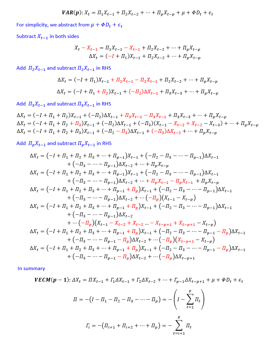
The Johansen cointegration test is applied to this this VECM(p-1) representation. Conversely, we can back out coefficients of VECM from that of VAR model using the above transformation.
Comparison of coefficients from VECM, cajorls, vec2var
In the previous post, the estimated parameters of vec2var() are somewhat different from that of the VECM() and cajorls() but I said that three sets of parameters are all the same. This is evident because we know the above transformation from VAR(p) to VECM(p-1).
Our example is about VECM(1) or VAR(2), we can convert parameters of vec2var() in the form of VECM representation as follows.
\[\begin{align} \Pi = -\left( I – \Pi_1 – \Pi_2 \right), \quad \Gamma_1 = -\Pi_2 \end{align}\]
The following R code implements these transformations.
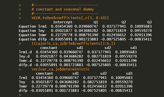
#—————————— # AR(1) #—————————— VECM_tsDyn$coefficients[,4:7] t(cajorls_ca.jo$rlm$coefficients[7:10,]) –vec2var_ca.jo$A$A2 #—————————— # ECT : long-run impact matrix #—————————— VECM_tsDyn$coefficients[,1:2] t(cajorls_ca.jo$rlm$coefficients[1:2,]) (vec2var_ca.jo$A$A1 + vec2var_ca.jo$A$A2 – diag(4))[,1:2] #—————————— # constant and seasonal dummy #—————————— VECM_tsDyn$coefficients[,c(3, 8:10)] t(cajorls_ca.jo$rlm$coefficients[3:6,]) vec2var_ca.jo$deterministic | cs |
AR(1) coefficients from three models are the same. (\(\Gamma_1 = -\Pi_2\))

Long-run impact matrices from three models are also the same. (\(\Pi = \Pi_1 + \Pi_2 – I\))

Intercepts and seasonal dummy variables are same as we found already in the previous post.
A Restricting Matrix
Before going to the Johansen’s hypothesis testing on parameter restrictions, we need to understand a restricting matrix and real parameters to be estimated.
Given an unrestricted parameter matrix \({\beta^u}\) with two columns which are considered two set of coefficients from two equations, a multiplication of some restricting matrix \(R\) and \({\beta^u}\) produces a restricted parameter matrix \({\beta^r}\).
| \[\begin{align} & \underbrace{\beta^r}_{v \times c} = \underbrace{R}_{v \times (v-r)} \times \underbrace{\beta^u}_{(v-r) \times c} \\\\ \color{blue}v &= \text{the number of }\color{blue}v\text{ariables} \\ \color{red}c &= \text{the number of }\color{red}c\text{ointegrations} \\ \color{green}r &= \text{the number of }\color{green}r\text{estrictions} \\ \end{align}\] |
In particular, when a restricting matrix does not have any restrictions, this restricting matrix coincides with the identity matrix as follows.
\[\begin{align} \underbrace{\begin{bmatrix} \beta^r_{11} & \beta^r_{12} \\ \beta^r_{21} & \beta^r_{22} \\ \beta^r_{31} & \beta^r_{32} \\ \beta^r_{41} & \beta^r_{42} \end{bmatrix}}_{\begin{matrix}{\text{restricted}}\\{\text{parameters}}\end{matrix}} = \ \underbrace{\begin{bmatrix} 1 & 0 & 0 & 0 \\ 0 & 1 &0 & 0 \\ 0 & 0 & 1 & 0 \\ 0 & 0 &0 & 1 \\ \end{bmatrix}}_{\begin{matrix}{\text{restricting}}\\{\text{matrix}}\end{matrix}} \underbrace{\begin{bmatrix} \beta^u_{11} & \beta^u_{12} \\ \beta^u_{21} & \beta^u_{22} \\ \beta^u_{31} & \beta^u_{32} \\ \beta^u_{41} & \beta^u_{42} \end{bmatrix}}_{\begin{matrix}{\text{unrestricted}}\\{\text{parameters}}\end{matrix}} \end{align}\] The resulting restricted parameters have the following representations. (i=1,2) \[\begin{align} \beta^r_{1i} &= \beta^u_{1i} \\ \beta^r_{2i} &= \beta^u_{2i} \\ \beta^r_{3i} &= \beta^u_{3i} \\ \beta^r_{4i} &= \beta^u_{4i} \end{align}\]
When we assume \(\beta^r_{2i} = 0\), the transformation between parameters have the following form. In this case, columns of a restricting matrix and rows of an unrestricted parameter matrix reduced by the number of restrictions (= 1) simultaneously.
\[\begin{align} \underbrace{\begin{bmatrix} \beta^r_{11} & \beta^r_{12} \\ \beta^r_{21} & \beta^r_{22} \\ \beta^r_{31} & \beta^r_{32} \\ \beta^r_{41} & \beta^r_{42} \end{bmatrix}}_{\begin{matrix}{\text{restricted}}\\{\text{parameters}}\end{matrix}} = \ \underbrace{\begin{bmatrix} 1 & 0 & 0 \\ 0 & 0 & 0 \\ 0 & 1 & 0 \\ 0 & 0 & 1 \\ \end{bmatrix}}_{\begin{matrix}{\text{restricting}}\\{\text{matrix}}\end{matrix}} \underbrace{\begin{bmatrix} \beta^u_{11} & \beta^u_{12} \\ \beta^u_{21} & \beta^u_{22} \\ \beta^u_{31} & \beta^u_{32} \\ \end{bmatrix}}_{\begin{matrix}{\text{unrestricted}}\\{\text{parameters}}\end{matrix}} \end{align}\] The resulting restricted parameters have the following representations. (i=1,2) \[\begin{align} \beta^r_{1i} &= \beta^u_{1i} \\ \beta^r_{2i} &= 0 \\ \beta^r_{3i} &= \beta^u_{2i} \\ \beta^r_{4i} &= \beta^u_{3i} \end{align}\]
Restrictions on Cointegrating Relationship
One advantage of Johansen’s approach is that it allows to easily test restrictions on \(\alpha\) and \(\beta\) with likelihood ratio test. These Hypothesis testings of restrictions on cointegrating relationship are carried out by alrtest(), blrtest() or ablrtest() functions in urca package.
In principle, one parameter restriction is on the corresponding coefficient of a variable. This leads to a selection matrix that determines which variable to be selected. In other words, parameter restrictions are performed not by setting \(\alpha\) and \(\beta\) matrices directly but by using the selection matrices indirectly. This selection matrix has the following form.
\[\begin{align} \Pi X_{t} &= \begin{bmatrix} \pi_{11} & \pi_{12} & \pi_{13} \\ \pi_{21} & \pi_{22} & \pi_{23} \\ \pi_{31} & \pi_{32} & \pi_{33} \end{bmatrix} \begin{bmatrix} x_{t} \\ y_{t} \\ z_{t} \end{bmatrix} \\ &= \begin{bmatrix} \alpha_{11} & \alpha_{12} \\ \alpha_{21} & \alpha_{22} \\ \alpha_{31} & \alpha_{32} \end{bmatrix} \begin{bmatrix} 1 & – \beta_{11} & – \beta_{12} \\ 1 & – \beta_{21} & – \beta_{22} \end{bmatrix} \begin{bmatrix} x_t \\ y_t \\ z_t \end{bmatrix} \\ &= \begin{bmatrix} \alpha_{11} & \alpha_{12} \\ \alpha_{21} & \alpha_{22} \\ \alpha_{31} & \alpha_{32} \end{bmatrix} \begin{bmatrix} 1 & 1 \\ – \beta_{11} & – \beta_{21} \\ – \beta_{12} & – \beta_{22} \end{bmatrix}^{‘} X_t \\ &= \alpha \beta^{‘} X_t \end{align}\]
1) Restrictions on beta
As in Johansen and Juselius (1990), the first hypothesis is that coefficients of money and income are equal with opposite sign as follows. \[\begin{align} H_3 : \beta_{1i} = -\beta_{2i} \end{align}\] This hypothesis can be represented in matrix notation. \[\begin{align} \underbrace{\begin{bmatrix} \beta^r_{11} & \beta^r_{12} \\ \beta^r_{21} & \beta^r_{22} \\ \beta^r_{31} & \beta^r_{32} \\ \beta^r_{41} & \beta^r_{42} \end{bmatrix}}_{\begin{matrix}{\text{restricted}}\\{\text{parameters}}\end{matrix}} = \ \underbrace{\begin{bmatrix} -1 & 0 & 0 \\ 1 & 0 & 0 \\ 0 & 1 & 0 \\ 0 & 0 & 1 \\ \end{bmatrix}}_{\begin{matrix}{\text{restricting}}\\{\text{matrix}}\end{matrix}} \underbrace{\begin{bmatrix} \beta^u_{11} & \beta^u_{12} \\ \beta^u_{21} & \beta^u_{22} \\ \beta^u_{31} & \beta^u_{32} \\ \end{bmatrix}}_{\begin{matrix}{\text{unrestricted}}\\{\text{parameters}}\end{matrix}} \end{align}\] The resulting restricted parameters have the following representations. (i=1,2) \[\begin{align} \beta^r_{1i} &= -\beta^u_{1i} \\ \beta^r_{2i} &= \beta^u_{1i} \\ \beta^r_{3i} &= \beta^u_{2i} \\ \beta^r_{4i} &= \beta^u_{3i} \end{align}\] We can use the following R code to apply this linear restriction on the cointegrating long run vector beta.
#———————————————- # Restrictions on beta matrix # H3 : beta=H*phi #———————————————- # Null Hypothesis ~ H3 : -b1 = b2 H <– matrix(byrow = TRUE, c(–1, 0, 0, 1, 0, 0, 0, 1, 0, 0, 0, 1), 4, 3) # Testing Hypothesis blr <– blrtest(coint_ca.jo, H=H, r=2) summary(blr) | cs |
In the above R code, the restriction matrix (H) has a dimension of 4×3 since there is one restriction and the number of parameters to be estimated is 6 (= 3×2) not 8 (= 4×2). Hypothesis testing on H3 null hypothesis is done by using blrtest() function in urca package.
2) Restrictions on alpha – weak exogeneity tests
The second hypothesis is that adjustment speeds of money and income are zero. This is so called the weak exogeneity test since when a speed of adjustment of some variable is zero, that variable does not be affected from the long-run cointegrating relationships.
\[\begin{align} H_4 : \beta_{1i} = 0 \text{ and } \beta_{2i} = 0 \end{align}\] This hypothesis can be represented in matrix notation. \[\begin{align} \underbrace{\begin{bmatrix} \beta^r_{11} & \beta^r_{12} \\ \beta^r_{21} & \beta^r_{22} \\ \beta^r_{31} & \beta^r_{32} \\ \beta^r_{41} & \beta^r_{42} \end{bmatrix}}_{\begin{matrix}{\text{restricted}}\\{\text{parameters}}\end{matrix}} = \ \underbrace{\begin{bmatrix} 0 & 0 \\ 0 & 0 \\ 1 & 0 \\ 0 & 1 \\ \end{bmatrix}}_{\begin{matrix}{\text{restricting}}\\{\text{matrix}}\end{matrix}} \underbrace{\begin{bmatrix} \beta^u_{11} & \beta^u_{12} \\ \beta^u_{21} & \beta^u_{22} \\ \beta^u_{31} & \beta^u_{32} \\ \end{bmatrix}}_{\begin{matrix}{\text{unrestricted}}\\{\text{parameters}}\end{matrix}} \end{align}\] The resulting restricted parameters have the following representations. (i=1,2) \[\begin{align} \beta^r_{1i} &= 0 \\ \beta^r_{2i} &= 0 \\ \beta^r_{3i} &= \beta^u_{1i} \\ \beta^r_{4i} &= \beta^u_{2i} \end{align}\] We can use the following R code to apply these two linear restrictions on the adjustment speed vector alpha.
#———————————————- # Restrictions on alpha matrix # – weak exogeneity tests # H4 : alpha=A*psi #———————————————- # Null Hypothesis ~ H4 : a1 = a2 = 0 A <– matrix(byrow = TRUE, c(0, 0, 0, 0, 1, 0, 0, 1), 4, 2) # Testing Hypothesis alr <– alrtest(coint_ca.jo, A=A, r=2) summary(alr) | cs |
In the above R code, the restriction matrix (A) has a dimension of 4×2 since there are two zero restrictions (weakly exogenous) and the number of parameters to be estimated is 4 (= 2×2) not 8 (= 4×2). Hypothesis testing on H4 null hypothesis is done by using alrtest() function in urca package.
3) Results of blrtest() and alrtest()
The following output is the concatenated two hypothesis testing results.
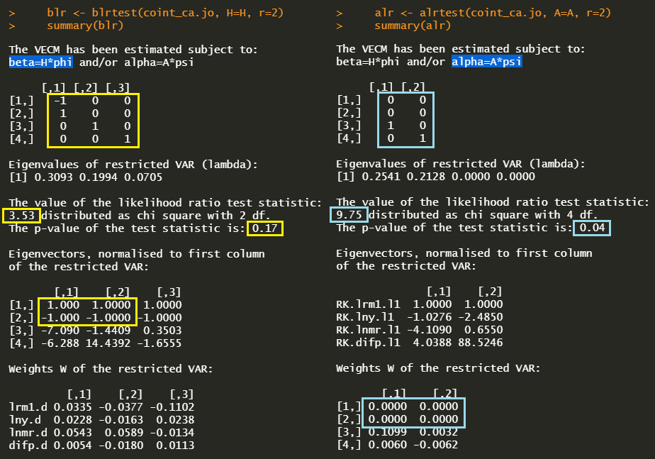
These results show that since p-value of H3 is 0.17, H3 hypothesis can not be rejected (beta restriction) under the 5% significant level. In contrast, H4 hypothesis is rejected (alpha restriction) since p-value of H4 is 0.04 under the 5% significant level. Therefore we can conclude that \(\beta_{1i} = -\beta_{2i}\) in cointegrating vectors and the first and second variables are not jointly weakly exogenous.
In summary, we can draw two conclusions.
|
Beta-restricted VECM
In VECM() function in tsDyn, user-defined beta (cointegrating vector) can be inserted into VECM() function with beta argument. The following R code implements a beta-restricted VECM model using the above blr output.
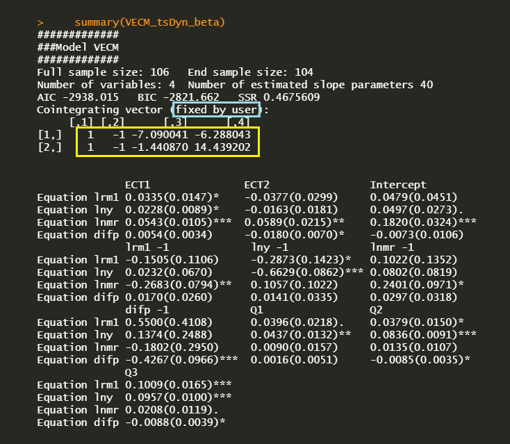
#======================================================== # Beta-restricted VECM #======================================================== VECM_tsDyn_beta <– VECM(lev, lag=1, r=2, estim = “ML”, LRinclude = “none”, exogen = dum_season, beta = blr@V[,1:2]) summary(VECM_tsDyn_beta) | cs |
The folloiwng result shows that VECM estimation is carried out, which is subject to user-defined beta cofficient matrix.
Concluding Remarks
In this post, we have dealt with some interesting issues regarding VECM model such as the hypothesis testing on parameter restrictions and the transformation of VAR(p) to VECM(p-1) and so on. In particular, as we have understood the concept of a restricting matrix, another various hypothesis testings are available using R by changing a restricting matrix.
Reference
Johansen, S. and Juselius, K. (1990), Maximum Likelihood Estimation and Inference on Cointegration – with Applications to the Demand for Money, Oxford Bulletin of Economics and Statistics, 52, 2, 169–210. \(\blacksquare\)
To leave a comment for the author, please follow the link and comment on their blog: K & L Fintech Modeling.
R-bloggers.com offers daily e-mail updates about R news and tutorials about learning R and many other topics. Click here if you're looking to post or find an R/data-science job.
Want to share your content on R-bloggers? click here if you have a blog, or here if you don't.