Bond Forward Pricing using R code
[This article was first published on K & L Fintech Modeling, and kindly contributed to R-bloggers]. (You can report issue about the content on this page here)
Want to share your content on R-bloggers? click here if you have a blog, or here if you don't.
This post presents a R code for pricing a bond forward. It is well known that insurance companies use it as the instrument of a duration management with lower cost. Here, a pricing formula and its implementation are provided with delta sensitivity using a zero curve bump-and-reprice approach. Want to share your content on R-bloggers? click here if you have a blog, or here if you don't.
Bond Forward Pricing
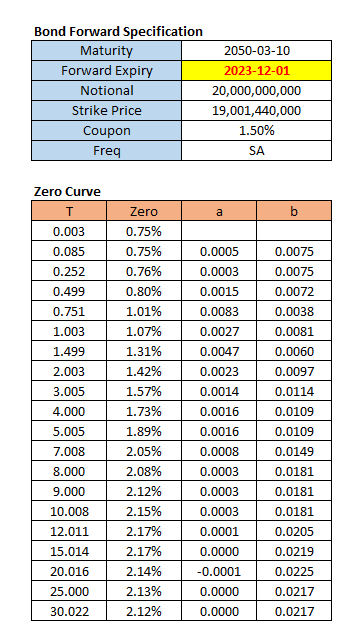
The bond forward contract is an agreement between two counterparties to exchange bonds at an agreed price (strike price) and time in the future (forward expiry). Let’s take the following example of 5 X 25 bond forward and a zero curve for discounting at Nov 21st, 2021 (pricing date).
Input Data
The input data for bond forward is a coupon rate for bond, a strike price, a zero curve, and so on.
In the above zero curve data, a and b denote \(\beta\) coefficient and constant term for a linear interpolation.
Bond Forward Pricing Formula
A Price of the bond forward (\(P(t)\)) is calculated by the difference between a sum of bond discounted cashflows after forward expiry and a discounted strike price.
\[\begin{align} P(t) &= DF(t_{fe})X – \sum_{t>t_{fe}}^{} {DF(t)*CF(t)} \\ X &: \text{strike price} \\ CF &: \text{bond cash flow} \\ DF &: \text{discount factor} \\ t_{fe} &: \text{date for forward expiry} \end{align}\]
We need to generate a stream of bond cash flows with linearly interpolated discount factor and calculate discounted cash flows.
Applying the above formula results in the following bond forward price (1,623,672,872)at at Nov 21st, 2021. \[\begin{align} P(t) &= DF(t_{fe})X – \sum_{t>t_{fe}}^{} {DF(t)*CF(t)} \\ &= 0.966418 \times 19,001,440,000 – 16,739,667,292 \\ &=1,623,672,872 \end{align}\]
R code
In the following R code, we interpolate a zero curve, calculate discounted cash flows and finally get a bond forward price.
1 2 3 4 5 6 7 8 9 10 11 12 13 14 15 16 17 18 19 20 21 22 23 24 25 26 27 28 29 30 31 32 33 34 35 36 37 38 39 40 41 42 43 44 45 46 47 48 49 50 51 52 53 54 55 56 57 58 59 60 61 62 63 64 65 66 67 68 69 70 71 72 73 74 75 76 77 78 79 80 81 82 83 84 85 86 87 88 89 90 91 92 | #========================================================# # Quantitative ALM, Financial Econometrics & Derivatives # ML/DL using R, Python, Tensorflow by Sang-Heon Lee # # https://kiandlee.blogspot.com #——————————————————–# # Bond Forward Pricing #========================================================# graphics.off() # clear all graphs rm(list = ls()) # remove all files from your workspace #—————————————————— # 1) Data #—————————————————— # NA, strike price, coupon rate notional_amount <– 20000000000 strike_price <– 19001440000 coupon_rate <– 0.015 # dates dt.pricing_date <– as.Date(“2021-09-27”) dt.next_coupon_date <– as.Date(“2022-03-10”) dt.forward_expiry <– as.Date(“2023-12-01”) dt.bond_maturity <– as.Date(“2050-03-10”) # input zero curve str.mat_zero <– “ mat zero 0.00274 0.007499920 0.084932 0.007544180 0.252055 0.007594760 0.49863 0.007969630 0.750685 0.010070770 1.00274 0.010744840 1.49863 0.013099340 2.00274 0.014240150 3.005479 0.015682820 4 0.017265780 5.005479 0.018866170 7.008219 0.020472420 8 0.020813900 9 0.021158210 10.008219 0.021505340 12.010959 0.021708300 15.013699 0.021667940 20.016438 0.021388380 25 0.021299100 30.021918 0.021209130 “ # input zero curve df.zr <– read.table(text = str.mat_zero, header = T) # linear interpolation fs<–approxfun(df.zr$mat, df.zr$zero); #—————————————————— # 2) cash flow table #—————————————————— # cash flow data.frame df <– data.frame( # cash flow schedule by 6 months date = seq(dt.next_coupon_date, dt.bond_maturity, “6 months”)) nr <– nrow(df) # a stream of maturity, cash flows, etc. df$mat <– as.numeric(julian(df$date, dt.pricing_date))/365 df$zero <– fs(df$mat) df$df <– exp(–df$mat*df$zero) df$cf <– (coupon_rate/2)*notional_amount df$cf[nr] <– df$cf[nr] + notional_amount df$dcf <– df$df*df$cf #—————————————————— # 3) Bond forward price #—————————————————— # maturity and zero rate mat <– as.numeric(julian(dt.forward_expiry, dt.pricing_date))/365 zero <– fs(mat) # print bond forward price –sum(df$dcf[df$date > dt.forward_expiry]) + exp(–mat*zero)*strike_price | cs |
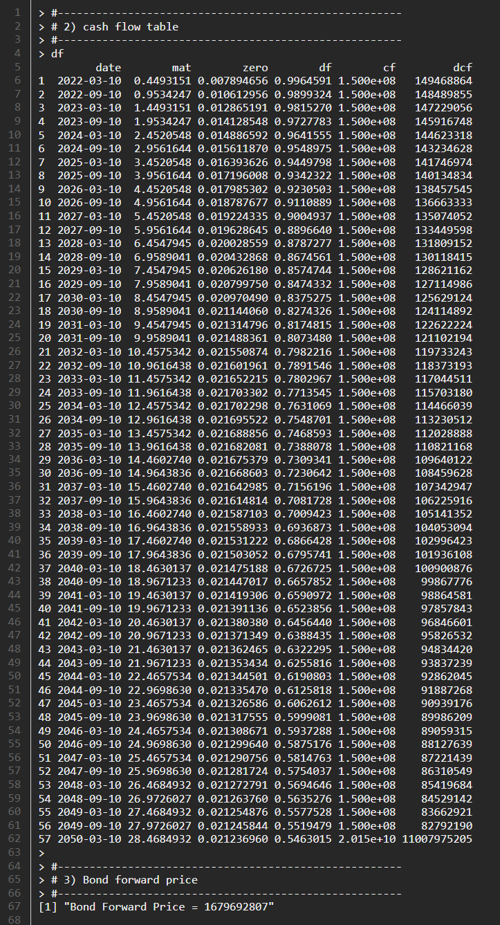
Running the above R code results in the following cash flow table and a price of the bond forward (1,679,692,807).
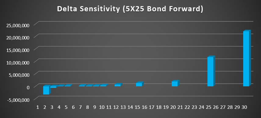
The next figures shows a delta sensitivity of 5 X 25 bond forward by using a zero curve bump-and-reprice method. The effect of strike price is negative and the effect of remaining bond cash flows are positive. To hedge this type of bond forward at inception, we should construct a delta-neutral portfolio by a purchase of 30Y bond and 5Y IRS pay. After constructing this initial hedged position, rebalancings and dynamic hedges for delta-neutral position are carried out periodically.
Concluding Remarks
In this post, we’ve implemented R code for pricing a bond forward which is widely used for duration management in insurance company. \(\blacksquare\)
To leave a comment for the author, please follow the link and comment on their blog: K & L Fintech Modeling.
R-bloggers.com offers daily e-mail updates about R news and tutorials about learning R and many other topics. Click here if you're looking to post or find an R/data-science job.
Want to share your content on R-bloggers? click here if you have a blog, or here if you don't.


