This post solves Adams and Deventer (1994) maximum smoothness forward rate curve as the matrix inversion of equality constrained quadratic programming problems. We implement R code for this model and elaborate on how to get monthly forward and spot rates from the calibrated parameters.

Maximum Smoothness Forward Rates

Using Adams and Deventer (1994, revised 2010) approach, output of this post is the following figure describing maximum smoothness forward rate curve with spot curve.


At first, details of maximum smoothness forward rate curve and the solution by using an optimization are explained in the previous post below.


We can solve Adams and Deventer (1994) maximum smoothness forward rate curve by matrix inversion. This solution is possible due to the fact that this problem can be formulated as the equality constrained quadratic programming problem.

Quadratic Programming with Linear Equality Constraints

Equality-constrained quadratic program (QP) is a QP where only linear equality constraints are present with quadratic terms absent.
\[\begin{align} &\min_{x}& &f(x) = \frac{1}{2}x^T Q x + c^T x \\ &s.t. & & Ax = b \end{align}\]
The first-order condition (FOC) for this problem constitutes the following linear system, which is derived from setting up the Lagrangian.
\[\begin{align} \underbrace{ \left[\begin{array}{ccc} Q & -A^T \\ A & 0 \\ \end{array}\right]}_{\text{KKT matrix}} \begin{bmatrix} x^* \\ \lambda^* \end{bmatrix} &= \begin{bmatrix} -c \\ b \end{bmatrix} \end{align}\] Here, matrix in LHS is called a KKT(Karush–Kuhn–Tucker) matrix. We can solve the above linear system by using the inverse matrix of the LHS coefficient matrix. The derivation of it is as follows.
Using Lagrange multiplier (\(\lambda\)), the optimization problems can be converted to the following Lagrangian. \[\begin{align} f(x,\lambda) = \frac{1}{2}x^T Q x + c^T x + \lambda^T(Ax – b) \end{align}\]
The FOC with respect to \(x\) and \(\lambda\) is
\[\begin{align} &\frac{\partial f(x,\lambda)}{\partial x} = Qx + c + A^T\lambda = 0 \\ &\frac{\partial f(x,\lambda)}{\partial \lambda} = Ax – b = 0 \end{align}\]
This two set of equations are reduced to the above vector-matrix representation and we use the inverse matrix of \(A\) to get an vector of optimal decision variables \(x\).
\[\begin{align} X = \begin{bmatrix} x^* \\ \lambda^* \end{bmatrix} &= \left[\begin{array}{ccc} Q & -A^T \\ A & 0 \\ \end{array}\right]^{-1} \begin{bmatrix} -c \\ b \end{bmatrix} \end{align}\]

Objecive Function

As can be seen in previous blog, these quadratic terms can be summarized as the following vector-matrix notation (\(\Delta t_i^n= t_i^n – t_{i-1}^n\)).
\[\begin{align} \int_{t_{i-1}}^{t_i} [f^{”}(t)]^2 dt = x_i^T Q_i x_i \end{align}\] where \[\begin{align} x_i = \begin{bmatrix} a_i \\ b_i \\ c_i \\ d_i \\ e_i \end{bmatrix}, Q_i = \left[\begin{array}{ccc} \frac{144}{5} \Delta t_i^5 & 18 \Delta t_i^4 & 8 \Delta t_i^3 & 0 & 0 \\ 18 \Delta t_i^4 & 12 \Delta t_i^3 & 6 \Delta t_i^2 & 0 & 0 \\ 8 \Delta t_i^3 & 6 \Delta t_i^2 & 4 \Delta t_i & 0 & 0 \\ 0 & 0 & 0 & 0 & 0 \\ 0 & 0 & 0 & 0 & 0 \\ \end{array}\right] \end{align}\]
Therefore, the objective function is the sum of i-th objective functions.
\[\begin{align} x^T Q x \end{align}\] where \[\begin{align} x = \begin{bmatrix} x_1 \\ x_2 \\ \vdots \\ x_{m-1} \\ x_m \end{bmatrix}, Q = \left[\begin{array}{ccc} Q_1 & 0 & … & 0 & 0 \\ 0 & Q_2 & … & 0 & 0 \\ \vdots & \vdots & \ddots & \vdots &\vdots \\ 0 & 0 & … & Q_{m-1} & 0 \\ 0 & 0 & … & 0 & Q_m \\ \end{array}\right] \end{align}\]
In this way, concatenation of the objective functions in each segment consist of \(Q\) matrix in the above QP.

Linear Equality Constraints

As can be seen also in previous blog, for \(\Delta k_{i+1}= k_{i+1} – k_{i}, \Delta t_i^n= t_i^n – t_{i-1}^n\), linear equality constraints are as follows.


1) continuity or smoothness at the joints (internal knots)\[\begin{align} 0 &= \Delta a_{i+1} t^4 + \Delta b_{i+1} t^3 + \Delta c_{i+1} t^2 + \Delta d_{i+1} t + \Delta e_{i+1} \\ 0 &= 4\Delta a_{i+1} t^3 + 3\Delta b_{i+1} t^2 + 2\Delta c_{i+1} t + d\Delta _{i+1} \\ 0 &= 12\Delta a_{i+1} t^2 + 6\Delta b_{i+1} t + 2\Delta c_{i+1} \\ 0 &= 24\Delta a_{i+1} t + 6\Delta b_{i+1} \end{align}\]
2) market price fitting at the observed points\[\begin{align} -log\left[ \frac{P_i}{P_{i-1}}\right] = \frac{1}{5} a_i \Delta t_i^5 + \frac{1}{4} b_i \Delta t_i^4 + \frac{1}{3} c_i \Delta t_i^3 + \frac{1}{2} d_i \Delta t_i^2 + e_i \Delta t_i \end{align}\]
2) Additional constraints for smoothness
\[\begin{align} f(0) = r(0), \quad f^{‘}(0) = 0 \\ f^{‘}(T) = 0 , \quad f^{”}(T) = 0 \end{align}\]
These linear equality constraints consist of \(A\) matrix in the above QP.

Fitting Yield Curve as a Quadratic Programming with Linear Equality Constraints

In our problem, the objective function consists of quadratic terms and the linear constraints are equality restrictions. Therefore, this can be represented as a equality-constrained QP.

\[\begin{align} \left[\begin{array}{ccc} Q & -A^T \\ A & 0 \\ \end{array}\right] \begin{bmatrix} x^* \\ \lambda^* \end{bmatrix} &= \begin{bmatrix} -c \\ b \end{bmatrix} \end{align}\] Using Adams and Deventer (2010) data, let’s construct left hand side KKT coefficient matrix and right hand side vector. The former consists of \(Q\), \(A\) and \(-A^T\) and the latter is made from \(b\) and \(-c\). Of course, the unknown \(X\) vector contains 25 coefficients of forward rate equations.

a1, b1, c1, d1, e1, a2, b2, c2, d2, e2, a3, b3, c3, d3, e3, a4, b4, c4, d4, e4, a5, b5, c5, d5, e5

Let’s construct three sub matrices : \(Q\), \(A\) and \(-A^T\).

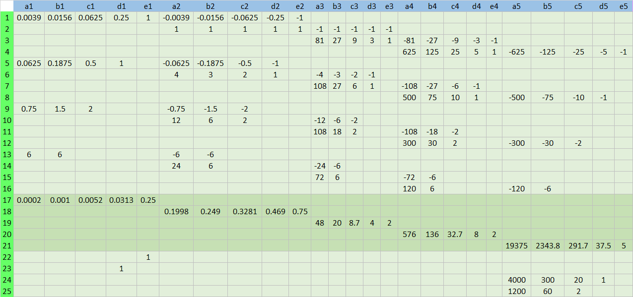
\(Q\) matrix is of the next form. For example, entry of (1,1) is 0.028125 = (144/5)*(0.25-0)^5. Values of remaining entries are calculated by using the objective function and constraints.

\(A\) matrix is of the following form.

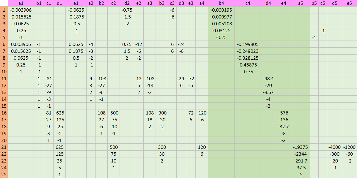
Its minus transpose, \(-A^T\) is

As vector \(c\) is a zero vector and vector \(b\) has some values which are derived from bond price matching conditions, the RHS vector consists of the following numbers.

0 , 0 , 0 , 0 , 0 , 0 , 0 , 0 , 0 , 0 , 0 , 0 , 0 , 0 , 0 , 0 , 0 , 0 , 0 , 0 , 0 , 0 , 0 , 0 , 0 , 0 , 0 , 0 , 0 , 0 , 0 , 0 , 0 , 0 , 0 , 0 , 0 , 0 , 0 , 0 , 0 , 0.012 , 0.033125 , 0.12 , 0.0975 , 0.3875 , 0.04 , 0 , 0 , 0


Finally, we can construct LHS coefficient matrix and RHS vector as follows.

As we know value of each entry, entries that have numerical value are colored black, blue and red. In LHS matrix, we display empty cells as zero values (0).

R code

The following R code implements the maximum smoothness forward curve by using an inverse matrix.



Running the above R code, we can obtain the following results which are the same as that of the previous post.

Monthly Spot and Forward Curves

As noted in the previous post, in a piece-wise linear form, the spot and forward rate are as follows.

\[\begin{align} f(t_i) &= a_i t^4 + b_i t^3 + c_i t^2 + d_i t + e_i \\ y(t_i) &= \frac{1}{t_i}\sum_{j=1}^{i}\left( \frac{1}{5} a_j \Delta t_j^5 + \frac{1}{4} b_j \Delta t_j^4 + \frac{1}{3} c_j \Delta t_j^3 + \frac{1}{2} d_j \Delta t_j^2 + e_j \Delta t_j \right) \end{align}\]
Using these equations, monthly forward rate and zero curve can be obtained by using the following R code.



Drawing spot and forward curve from the maximum smoothness principle results in the following figure. These spot curve is market consistent as it fits market spot rates exactly. The forward curve shows very smooth behavior.

Shortcut Method

In this problem, I guess that we can use \(x = A^{-1}b\) as shortcut method. It is because of the fact that as \(x\) is determined by \( Ax – b \rightarrow x = A^{-1}b \), \(\lambda\) vector is determined by some arbitrary \(Q\) matrix except for the zero or null matrix.
\[\begin{align} Qx + A^T\lambda = 0 \rightarrow \lambda = (A^T)^{-1}Qx \end{align}\]
In the above equation, if \(A\) and \(x\) are known, even though we use non-zero some arbitrary \(Q\) matrix, we can get the same \(x\) with different \(\lambda\). I think this is due to the fact that our problem is exactly identified with only linear equality constraints and there is no perturbation process. The following R code consists of the linear system solution by using inverse of sub matrix \(mA\) not \(A\).




Lagrange multiplier is important concept as it is interpreted as shadow price or marginal utility in financial economics. But in the yield curve fitting context, it is of less significance. If there is no additional constraints and our purpose is to obtain only \(x\), I think it suffice to solve \(Ax = b\). Of course if we impose additional constraints, this shortcut will be impossible. This argument is my guess so that it is subject to correction if any inconsistency is found.

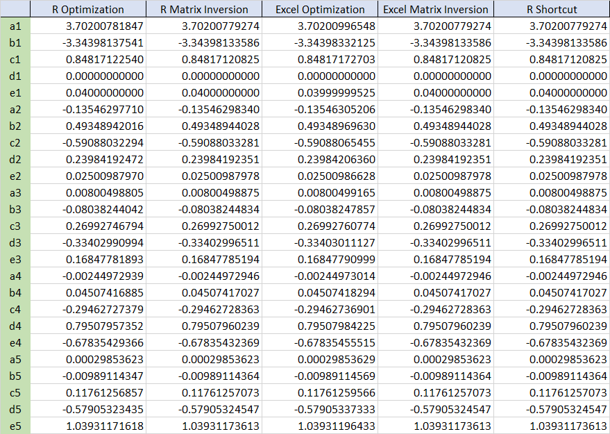
Finally, we compare forward curves from 1) R optimization, 2) Excel optimization, 3) R matrix inversion, 4) Excel matrix inversion, 5) R shortcut method. As we use Excel to illustrate the structure of sub and whole matrix or vector, coefficients can be found by using Excel solver.

The following table shows that there are negligible differences among estimated coefficients from 5 methods in the numerical perspective.

Concluding Remarks

From this post, we have implemented Adams and Deventer’s maximum smoothness forward curve. This powerful method will be used for various area, for example, interest rate trading desk since this department have a need to use exact and smooth forward curve. \(\blacksquare\)