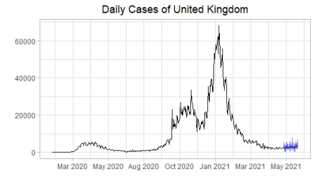
In the previous article, we examined the performances of covid-19 management of some developed countries and we found that the UK was slightly better than others. This time we are going to predict the spread of disease for about a month in the UK. The algorithm we will use for this purpose is the neural network.

Neural Network Structure

The neural network consists of three layers. The predictors form the bottom layer, the predicted output form the top layer and, the ones of the middle between them form the intermediate layers called the hidden neurons.

As we can see from the above graph, each layer of intermediate nodes takes the input from the previous layer. Each node and corresponding weight coefficients are combined in linear regression. Because of the hidden neurons(j), the output is recalculated by a nonlinear function. This is called the multilayer feed-forward network.

As mentioned before, the output is recalculated by the sigmoid function, which is nonlinear.

The modified output is given to the next layer as an input. This process is useful for the network to be robust to outliers. The weights () are randomly chosen and then learn from the observations by minimizing the cost function (e.g. MSE).

In time series regression, lagged values of data are used as input by a neural network, which is called the neural network autoregression(NNAR). We will use feed-forward with one hidden layer, which is denoted NNAR(p, k). p indicates lagged values, and k denotes the nodes in the hidden layer.

For seasonal time series, it is better to include that the last observation from the same term from the previous year. In this case, it is denoted as indicates that:

• for the lagged inputs(predictors).
• for the seasonal terms.

For non-seasonal time series data, the default p value is determined by the optimal number of lagged inputs according to the Akaike’s information criterion.

• T is the number of observations.
• SSE: sum of the squared of errors.
• k is the number of predictors.

If k is not selected at first, it is determined as . The network repeats 20 times as default and is trained for starting points which are different random weights. All the results are averaged for ultimate output. The process uses lagged values as inputs for a one-step forecast. This forecast along with the lagged values is used to predict a two-step forecast. This process continues until it meets the required forecasts.

We will prefer the non-seasonal approach because the data we will be using is less than the two periodic cycles required for detecting seasonality. We are going to predict daily cases in the UK for the next 30 days. The data file(covid_uk.csv) can be downloaded from here.

library(tidyverse)
library(forecast)
library(purrr)
library(lubridate)


#Building the dataframe
df <- read_csv("covid_uk.csv", 
               col_types = list(col_character(),
                                col_date(format = "%d/%m/%Y"),
                                col_double()))

#Converting to the time series data
inds <- seq(as.Date("2020-01-31"), as.Date("2021-05-21"), by = "day")
df_ts <- df %>%
  .$new_cases %>% 
  ts(start = c(2020, as.numeric(format(inds[1], "%j"))),frequency = 365)

Before modeling the data, we will use bootstrap aggregating to prevent overfitting and improve accuracy. This process has been detailed in one of the previous articles. We will make a function to predict, and show the results in a plot, but before doing that, we create a date transform variable to be used for readable dates.

#The function to convert decimal date to the proper format
date_transform <- function(x) {format(date_decimal(x), "%b %Y")}


#Forecasting with Simulated Neural Network and plotting the results
sim_nn <-  function(data, freq, h, n=100){
  
  #For reproducible results
  set.seed(123)
  
  #Bootstraping the time series
  sim <- bld.mbb.bootstrap(data, n)
  
  #Bagged Neural Network
  future <- sim %>% 
    map(function(x){simulate(nnetar(x, P=0),nsim=h)}) %>% 
    unlist() %>% 
    matrix(ncol = h, nrow = n, byrow = TRUE) %>% 
    pmax(0)#preventing the negative values
  
  #The beginning date of the prediction  
  start <- tsp(data)[2]+1/freq
  
  #Forecast object with prediction intervals 
  #at %5 significance level
  sim_fc <- structure(list(
    mean = ts(colMeans(future), start=start, frequency=freq),
    
    lower = future %>% as.data.frame() %>% 
      map_dbl(quantile, prob = 0.025) %>% 
      ts(start = start,frequency = freq),
    
    
    upper = future %>% as.data.frame() %>% 
      map_dbl(quantile, prob = 0.975) %>% 
      ts(start = start,frequency = freq),
    
    
     level=95),
    class="forecast")
  
  #Making predictions global variable for easy access
  assign("simfc",simfc,envir = .GlobalEnv)
  
 #Plotting the prediction results with the observations 
 sim_plot <-  autoplot(data)+ 
    autolayer(simfc)+
    scale_x_continuous(labels = date_transform,breaks = seq(2020,2022,0.2))+
    ylab("")+xlab("")+
    ggtitle("Daily Cases of United Kingdom")+
    theme_light()+
    theme(plot.title = element_text(hjust = 0.5))
 
 #Converting time series with decimal date
 #to the dataframe for proper demonstration
 start <- start %>% as.numeric() %>% date_decimal() %>%  as.Date()
 h_date <- seq(start, start+29, by = "day") 
 simfc_df <- simfc %>% data.frame()
 rownames(simfc_df)<- h_date
 
 #The output list
 list(simfc_df,sim_plot)
  
}


sim_nn(df_ts,365,30)

References

• Forecasting: Principles and Practice, Rob J Hyndman and George Athanasopoulos
• Our World in Data