Automatically Detecting Corners on Rally Stage Routes Using R
Want to share your content on R-bloggers? click here if you have a blog, or here if you don't.
One of the things I’ve started pondering with my rally stage route metrics is the extent to which we might be able to generate stage descriptions of the sort you might find on the It Gets Faster Now blog. The idea wouldn’t necessarily be to create finished stage descriptions, more a set of notes that a journalist or fan could use as a prompt to create a more relevant description. (See these old Notes on Robot Churnalism, Part I – Robot Writers for a related discussion.)
So here’s some sketching related to that: identifying corners.
We can use the rLFT (Linear Feature Tools) R package to calculate a convexity measure at fixed sample points along a route (for a fascinating discussion of the curvature/convexity metric, see *Albeke, S.E. et al. Measuring boundary convexity at multiple spatial scales using a linear ‘moving window’ analysis: an application to coastal river otter habitat selection Landscape Ecology 25 (2010): 1575-1587).
By filtering on high absolute convexity sample points, we can do a little bit of reasoning around the curvature at each point to make an attempt at identifying the start of a corner:
library(rLFT)

stepdist = 10
window = 20
routeConvTable <- bct(utm_routes[1,],
                      # distance between measurements
                      step = stepdist,
                      window = window, ridName = "Name")

head(routeConvTable)
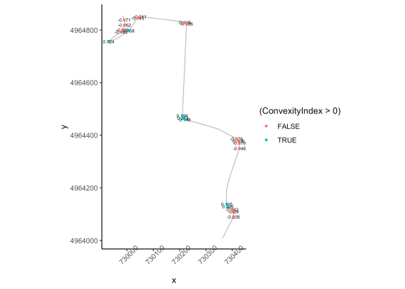
We can then use the convexity index to highlight the sample points with a high convexity index:
corner_conv = 0.1

tight_corners = routeConvTable[abs(routeConvTable$ConvexityIndex)>corner_conv,]
tight_corners_zoom1 = tight_corners$Midpoint_Y>4964000 & tight_corners$Midpoint_Y<4965000

ggplot(data=trj[zoom1, ],
       aes(x=x, y=y)) + geom_path(color='grey') + coord_sf() +
  geom_text(data=tight_corners[tight_corners_zoom1,],
                           aes(label = ConvexityIndex,
                               x=Midpoint_X, y=Midpoint_Y),
                           size=2) +
  geom_point(data=tight_corners[tight_corners_zoom1,],
             aes(x=Midpoint_X, y=Midpoint_Y,
                 color= (ConvexityIndex>0) ), size=1) +
  theme_classic()+
  theme(axis.text.x = element_text(angle = 45))

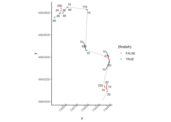
We can now do a bit of reasoning to find the start of a corner (see Automatically Generating Stage Descriptions for more discussion about the rationale behind this):
cornerer = function (df, slight_conv=0.01, closeby=25){
  df %>%
    mutate(dirChange = sign(ConvexityIndex) != sign(lag(ConvexityIndex))) %>%
    mutate(straightish =  (abs(ConvexityIndex) < slight_conv)) %>%
    mutate(dist =  (lead(MidMeas)-MidMeas)) %>%
    mutate(nearby =  dist < closeby) %>%
    mutate(firstish = !straightish &
                        ((nearby & !lag(straightish) & lag(dirChange)) |
                        # We don't want the previous node nearby
                        (!lag(nearby)) )  & !lag(nearby) )
}

tight_corners = cornerer(tight_corners)
Let’s see how it looks, labeling the points as we do so with the distance to the next sample point:
ggplot(data=trj[zoom1,],
       aes(x=x, y=y)) + geom_path(color='grey') + coord_sf() +
  ggrepel::geom_text_repel(data=tight_corners[tight_corners_zoom1,],
                           aes(label = dist,
                               x=Midpoint_X, y=Midpoint_Y),
                           size=3) +
  geom_point(data=tight_corners[tight_corners_zoom1,],
             aes(x=Midpoint_X, y=Midpoint_Y,
                 color= (firstish) ), size=1) +
  theme_classic()+
  theme(axis.text.x = element_text(angle = 45))

In passing, we note we can identify the larg gap distances as "straights" (and then perhaps look for lower convexity index corners along the way we could label as "flowing" corners, perhaps).
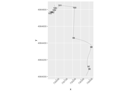
Something else we might do is number the corners:

There’s all sorts of fun to be had here, I think!
R-bloggers.com offers daily e-mail updates about R news and tutorials about learning R and many other topics. Click here if you're looking to post or find an R/data-science job.
Want to share your content on R-bloggers? click here if you have a blog, or here if you don't.
