I started my career in finance in 2007. For about a year I thought “this is great!” Then 2008 hit and I thought “this is terrible!”

After 2008, I had one fundamental question that I wanted answered: how much can you lose in an investment portfolio before you’ve lost too much? After about five years of research I realized that no one had an answer to this question. I had already started to develop my own, and this ultimately culminated in my first academic publication “Quantifying Downside Risk in Goal-Based Portfolios.” I subsequently expanded the ideas in a later publication “The Erosion of Portfolio Loss Toelrance Over Time: Defining, Defending, and Discussing.”

Here I want to simply present the ideas and how you can execute them using R. If you want the fuller theory, I’d suggest reading the publications themselves!

For this post, we’ll need the following libraries

library(tidyverse)
library(quantmod)

DEFINING PORTFOLIO LOSS TOLERANCE
First, we need to define unrecoverable losses. The point at which a portfolio cannot be reasonably expected to recover is pretty simple (if we exclude contributions):

where V is the required future value of your portfolio, v is the current value of your portfolio, R is the recovery return you can expect from your portfolio, and t is the time until you need the money. Given these variables, this is the maximum loss you can sustain in the coming period.

Let’s convert this into an R function for use later.

mal.f <- function(current_value, future_value, time, recovery_return){
  future_value / (current_value * (1 + recovery_return)^(time - 1)) - 1
}

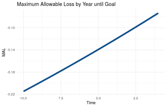
If we plot the function, keeping time as the variable and assuming our portfolio grows at the expected rate every year, we can see that your maximum loss tolerance erodes every year. Time, it turns out, is the most critical variable in your risk-tolerance.

# Define the variables
time <- seq(10, 1, -1)
current_value <- 0.50 * (1.08)^time %>% rev()
future_value <- 1
recovery_return <- 0.10
# Load variables into a data frame and pipe into a ggplot
data.frame( "Time" = time,
            "MAL" = mal.f(current_value,
                          future_value,
                          time,
                          recovery_return) ) %>% 
  ggplot( ., aes( x=Time, y=MAL) )+
  geom_line(size=2, col='dodgerblue4' )+
  scale_x_reverse()+
  labs(title = 'Maximum Allowable Loss by Year until Goal')+
  theme_minimal()

Yielding

MANAGING YOUR LOSS TOLERANCE
Now that we know what your loss tolerance is, we can go about managing it.

The first and most obvious way we can control downside risk is through hedging and stop-losses. This is the method that can help ensure you don’t exceed your risk budget in any given year. Hedging, however, doesn’t help you manage your loss tolerance through time. I won’t really go into this topic here because hedging is a whole other animal.

The second and more potent way to manage your risk tolerance is through portfolio allocation (i.e. stock/bond/alternatives allocation). Interestingly, taking more stock risk gives you more tolerance for risk both today and at the end of your portfolio’s life. This is because you develop excess return as the portfolio moves through time.

Let’s demonstrate this through an example. We are going to pull actual stock and bond data, then build simple stock/bond portfolios. From there, we can generate a return expectation for each portfolio and a recovery expectation for each portfolio. For my recovery expectations, I prefer the 60th percentile of returns. That is better than average, but not dependent on the absolute best returns we’ve ever seen. See below for the code and comments.

# Pull historical stock and bond returns
getSymbols( c('SPY', 'AGG'), from='2004-01-01', to='2020-08-16')

# Convert data to monthly returns
stock_return <- SPY$SPY.Adjusted[xts:::startof(SPY$SPY.Adjusted, 'months')] %>% 
  Delt()
bond_return <- AGG$AGG.Adjusted[xts:::startof(AGG$AGG.Adjusted, 'months')] %>% 
  Delt()

# Set up potential portfolios
stock_allocation <- seq(0, 1, 0.01)
bond_allocation <- 1 - stock_allocation
portfolio_mean_return <- (stock_allocation * mean( na.omit( stock_return ) ) + 
                            bond_allocation * mean( na.omit( bond_return ) ) ) * 12

# Find recovery returns for each portfolio.
# I chose the 60th percentile of returns as a recovery expectation
portfolio_recovery_return <- 0
for(i in 1:length(stock_allocation)){
  portfolio_recovery_return[i] <- quantile(
    (stock_allocation[i] * na.omit(stock_return) +
    bond_allocation[i] * na.omit(bond_return) ) * 12, 0.6 )
}

# Now build a matrix of maximum allowable losses (MAL), simulating 
# portfolio growth at the expected return rate for each portfolio
# allocation.
years <- seq(1, 10, 1)
current_value <- 0
MAL.m <- matrix( nrow = length(portfolio_mean_return),
                 ncol = length(years) )
for(i in 1:length(portfolio_mean_return)){
  for(j in 1:length(years)){
    current_value <- 0.6 * (1 + portfolio_mean_return[i])^rev(years)[j]
    MAL.m[i,j] <- mal.f( current_value, 1, years[j], portfolio_recovery_return[i])
  }
}

# Visualize the result.
persp(x = stock_allocation,
      y = years,
      z = MAL.m,
      theta = 50,
      phi = 10,
      main = 'Maximum Allowable Loss',
      xlab = '% Stock Allocation',
      ylab = 'Years Until Goal',
      zlab = 'MAL',
      ticktype = 'detailed')

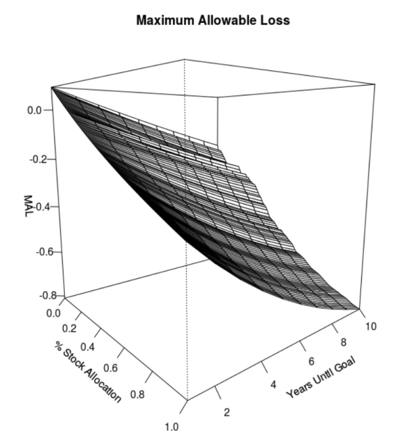
The visualization yields a perspective plot. As you can see, in this example, a stock-heavy allocation gives you considerably more loss-tolerance both early in your portfolio’s life (i.e. 10-years until goal) as well as later (i.e. 1-year until goal). This result was confirmed from a different perspective in some of my later research.

Of course, that may not be the case in every scenario, but it is generally true for non-aspirational goals that are more than about five years out.

In fact, if you optimize your portfolio using a goals-based methodology, your loss-tolerance is automatically optimized, too. I will do a later post on goals-based portfolio optimization, but for now you at least have an understanding of how to think about the problem.