The tsbox package makes life with time series in R easier. It is built around a set of functions that convert time series of different classes to each other. They are frequency-agnostic, and allow the user to combine time series of multiple non-standard and irregular frequencies. A detailed overview of the package functionality is given in the documentation page (or in a previous blog-post).

Version 0.2 is now on CRAN and provides a larger number of bugfixes. Non-standard column names are now handled correctly, and non-standard column orders are treated consistently.

New Classes

There are two more time series classes supported: tis time series, from the tis package, and irts time series, from the tseries package.

In order to create an object of these classes, it is sufficient to use the appropriate converter.

E.g., for tis time series:

library(tsbox)
ts_tis(fdeaths) 

##       Jan  Feb  Mar  Apr  May  Jun  Jul  Aug  Sep  Oct  Nov  Dec
## 1974  901  689  827  677  522  406  441  393  387  582  578  666 
## 1975  830  752  785  664  467  438  421  412  343  440  531  771 
## 1976  767 1141  896  532  447  420  376  330  357  445  546  764 
## 1977  862  660  663  643  502  392  411  348  387  385  411  638 
## 1978  796  853  737  546  530  446  431  362  387  430  425  679 
## 1979  821  785  727  612  478  429  405  379  393  411  487  574 
## class: tis 

Or for irts time series:

head(ts_irts(fdeaths)) 

## 1974-01-01 00:00:00 GMT 901 
## 1974-02-01 00:00:00 GMT 689 

Conversion works from all classes to all classes, and we can easily convert these objects to any other time series class, or to a data frame:

x.tis <- ts_tis(fdeaths) 
head(ts_df(x.tis)) 

##         time value 
## 1 1974-01-01   901 
## 2 1974-02-01   689 
## 3 1974-03-01   827 
## 4 1974-04-01   677 
## 5 1974-05-01   522 
## 6 1974-06-01   406 

Class-agnostic functions

Because coercion works reliably and is well tested, we can use it to make functions class-agnostic. If a class-agnostic function works for one class, it works for all:

ts_pc(ts_tis(fdeaths)) 
ts_pc(ts_irts(fdeaths)) 
ts_pc(ts_df(fdeaths)) 
ts_pc(fdeaths) 

ts_pc calculates percentage change rates towards the previous period. It works like a ‘generic’ function: You can apply it on any time series object, and it will return an object of the same class as its input.

So, whether we want to smooth, scale, differentiate, chain-link, forecast, regularize or seasonally adjust a series, we can use the same commands to all time series classes. tsbox offers a comprehensive toolkit for the basics of time series manipulation. Here are some additional examples:

ts_pcy(fdeaths)                # pc., comp. to same period of prev. year 
ts_forecast(fdeaths)           # forecast, by exponential smoothing 
ts_seas(fdeaths)               # seasonal adjustment, by X-13 
ts_frequency(fdeaths, "year")  # convert to annual frequency 
ts_span(fdeaths, "-1 year")    # limit time span to final year 

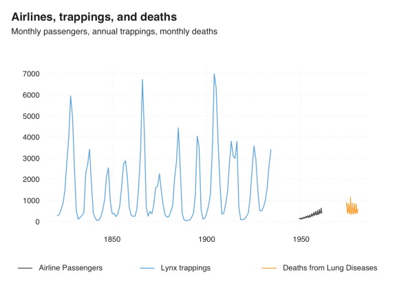
There are many more. Because they all start with ts_, you can use auto-complete to see what’s around. Most conveniently, there is a time series plot function that works for all classes and frequencies:

ts_plot(
   `Airline Passengers` = AirPassengers,
   `Lynx trappings` = ts_tis(lynx),
   `Deaths from Lung Diseases` = ts_xts(fdeaths),
   title = "Airlines, trappings, and deaths",
   subtitle = "Monthly passengers, annual trappings, monthly deaths" 
)