Remember Magic Eye pictures? It was a craze in the 1990s where you would get books of abstract Pollockesque images, and, using a special technique, you could see a “3D” image. The technique, which I could never properly master, was to see “through” the page, focusing your gaze on a point behind the paper. The images are constructed in a such a way that that a subtly repeating pattern in the splodges tricked your brain into seeing the flat swirls of colour as contoured, and shapes would loom out of the paper.

I never quite mastered it, in the sense that I could only do it by crossing my eyes, meaning I was focusing in front of the page. It was effective in a sense: I could see three dimensional images, but they were recessed into the page instead of leaping off the page towards me.

This puzzle has its coordinates hidden in a magic eye picture. And I thought: what about those who’ve never mastered the art of magicking the hidden shapes off the page? I’m sure that’s something we can achieve with R, right?

The key to this is understanding that the image is largely a repeating horizontal pattern. The subtle differences are what gives us the 3D effect, but underpinning it is a regular pattern that we can exploit. If we can overlay two versions of the same image, offset horizontally by just the right amount, the difference between them should give us an image of the hidden shapes.

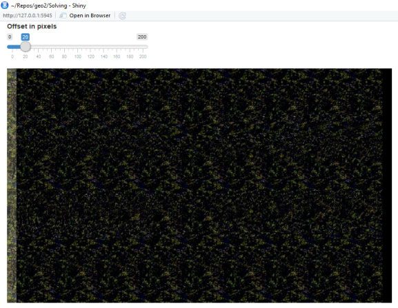
I could have sought to automatically detect the optimum distance — and that would still make a fascinating task some day — but I chose what felt to me the easier option. I built a Shiny package with a simple slider where the user specifies the offset, in pixels. Beneath that, an image dynamically shows the difference between images.

I had to consult the help files for renderImage and I was a bit worried that the process might be a bit clunky, since the jpg matrix is saved as a file which is then reloaded into the app. That read-write overhead seemed like a potential bottleneck, but when I ran it it responded well. Furthermore, the temporary file it creates each time the slider is adjusted is deleted straight after rendering, meaning I didn’t create digital clutter.

Here’s the start state of the app. The image is totally black because the two copies are aligned, and there is no difference.:

As I shift the slider along, I watch the patterns rising and falling…

Here’s the full code:

library(shiny)
library(jpeg)
library(abind)
magic <- readJPEG("c:/Users/alunh/OneDrive/Documents/Repos/geo2/Solving/GCTV41_magic-eye-view.jpg")
ui <- fluidPage(
  sliderInput(inputId = "offset", label = "Offset in pixels", min = 0, max = 200, value = 0, step = 1),
  imageOutput(outputId = "imag", height = "300px")
)
server <- function(input, output, session) {
  output$imag <- renderImage({     
    offset <- input$offset      
    magic1 <- magic %>% abind(array(0, replace(dim(magic), 2, offset)), along = 2)
    magic2 <- magic %>% abind(array(0, replace(dim(magic), 2, offset)), ., along = 2)
    magicdiff <- magic1 - magic2
    outfile <- tempfile(fileext='.jpg')
    writeJPEG(magicdiff, outfile)
    list(src=outfile, alt="..magic!")
  })
}
shinyApp(ui, server)

Yeah, that’s pretty minimal for something so powerfully interactive. Shiny is not without its flaws, but it does the heavy lifting for you if you want a quick interactive app, and it’s a major selling point for the R programming language.

Here’s the final image, where you can just see the N51 and W002 start of the final coordinates. I hidden the full solution out of respect to the cache owner.