Geelong and the curse of the bye
Want to share your content on R-bloggers? click here if you have a blog, or here if you don't.
This week we return to Australian Rules Football, the R package fitzRoy and some statistics to ask – why can’t Geelong win after a bye?
(with apologies to long-time readers who used to come for the science)
Code and a report for this blog post are available at Github.
First, some background. In 2011 the AFL expanded from 16 to 17 teams with the addition of the Gold Coast Suns. In the same year, a bye round (a week where some teams don’t play) was reintroduced to the competition. For the purposes of this discussion, we are interested only in bye rounds since 2011, and during the regular home/away season.
You will often hear footy fans claim – sometimes with very little evidence – that “we don’t go well after the bye.” For one team, this is certainly true. That team is Geelong, who have not won a game in the round following a bye since Round 7 in 2011.
Is this unusual? If so, does the available game data suggest any reason?
We start as ever with the excellent fitzRoy package and use get_match_results() to – well, get the match results.
Next, we can use some tidyverse magic to obtain all games in the round immediately before, and after, a bye. This looks long and complicated, so here’s an version with annotations in the comments to explain what’s going on:
results_bye <- results %>%
  # choose the desired columns
  select(Season, Round, Date, Venue, Home.Team, Away.Team, Margin) %>%
  # create one column for teams, another to indicate whether home or away
  gather(Status, Team, -Season, -Round, -Margin, -Date, -Venue) %>%
  # filter for 2011 onwards and only home/away games
  filter(Season > 2010, grepl("^R", Round)) %>%
  # create a column with the number of each round
  separate(Round, into = c("prefix", "suffix"), sep = 1) %>%
  mutate(suffix = as.numeric(suffix)) %>%
  # for each team's games in a season find games
  # the week before and after a bye
  arrange(Season, Team, suffix) %>%
  group_by(Season, Team) %>%
  mutate(bye = case_when(
    suffix - lead(suffix) == -2 ~ "before",
    suffix - lag(suffix) == 2 ~ "after",
    TRUE ~ as.character(suffix)
  ),
  # margins are with respect to home team so negate them if away
  Margin = ifelse(Status == "Away.Team", -Margin, Margin)) %>%
  ungroup() %>%
  # filter for the pre- and post-bye games
  filter(bye %in% c("before", "after")) %>%
  # calculate result
  mutate(Result = case_when(
    Margin > 0 ~ "W",
    Margin < 0 ~ "L",
    TRUE ~ "D"
  )) %>%
  # recreate the Round column
  unite(Round, prefix, suffix, sep = "")
Let’s confirm that Geelong have not won after a bye in a long time:
results_bye %>%
  filter(Team == "Geelong", bye == "after")
| Season | Round | Date | Venue | Margin | Status | Team | bye | Result |
|---|---|---|---|---|---|---|---|---|
| 2011 | R7 | 2011-05-07 | Kardinia Park | 66 | Home.Team | Geelong | after | W |
| 2011 | R23 | 2011-08-27 | Kardinia Park | -13 | Home.Team | Geelong | after | L |
| 2012 | R13 | 2012-06-22 | S.C.G. | -6 | Away.Team | Geelong | after | L |
| 2013 | R13 | 2013-06-23 | Gabba | -5 | Away.Team | Geelong | after | L |
| 2014 | R9 | 2014-05-17 | Subiaco | -32 | Away.Team | Geelong | after | L |
| 2016 | R16 | 2016-07-08 | Kardinia Park | -38 | Home.Team | Geelong | after | L |
| 2017 | R13 | 2017-06-15 | Subiaco | -13 | Away.Team | Geelong | after | L |
| 2018 | R15 | 2018-06-29 | Docklands | -2 | Away.Team | Geelong | after | L |
| 2019 | R14 | 2019-06-22 | Adelaide Oval | -11 | Away.Team | Geelong | after | L |
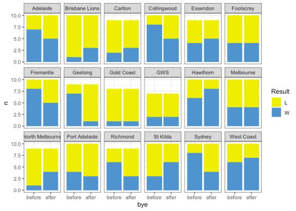
How does that compare with other teams?
We see all combinations: teams that seem to win more after a bye, as well as teams that win less and teams for which a bye makes no difference. However, Geelong certainly has the worst post-bye win/loss record.
We can ask: is the win/loss count in pre-bye games significantly different to those post-bye? One approach to this is to construct 2×2 contingency tables and perform Fisher’s exact test.
With some more tidyverse magic we can nest the data for each team, generate the tests and summarise the results. This approach is explained very nicely in “Running a model on separate groups” over at Simon Jackson’s blog.
Only Geelong has p < 0.05, suggesting that there is something interesting about the win/loss count after the bye. We’ll just show the first 5 teams here.
results_bye %>%
  count(Team, bye, Result) %>%
  nest(-Team) %>%
  mutate(data = map(data, . %>% spread(Result, n) %>% select(2:3)),
         fisher = map(data, fisher.test),
         summary = map(fisher, tidy)) %>%
  select(Team, summary) %>%
  unnest() %>%
  select(-method, -alternative) %>%
  arrange(p.value) %>%
  pander(split.table = Inf)
| Team | estimate | p.value | conf.low | conf.high |
|---|---|---|---|---|
| Geelong | 21.4 | 0.01522 | 1.533 | 1396 |
| Sydney | 5.43 | 0.1698 | 0.6027 | 79.83 |
| North Melbourne | 0.1736 | 0.2941 | 0.002835 | 2.438 |
| Richmond | 3.68 | 0.3469 | 0.4059 | 43.34 |
| Collingwood | 3.719 | 0.3498 | 0.4048 | 53.81 |
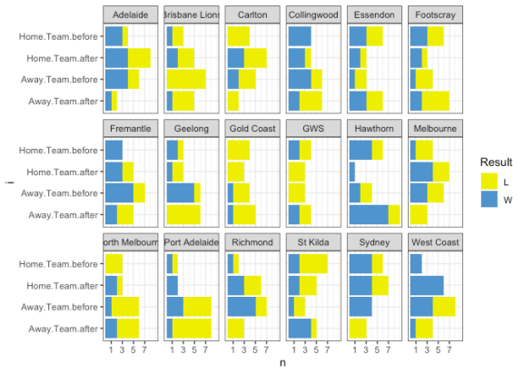
We can extend the previous visualisation by further breaking down games into home and away:
Now we see that of Geelong’s 8 post-bye losses, 6 were away games. Port Adelaide have a similar record. Then again, Brisbane have not won an away game before the bye, but you don’t hear anyone talking about Brisbane “not going well before the bye”.
When we look at those 6 away post-bye losses, one was in Melbourne – which in terms of travel distance is not very far from Geelong. The other five were “genuine” away games in Sydney, Brisbane, Adelaide and Perth (2).
| Season | Round | Date | Venue | Margin | Status | Team | bye | Result |
|---|---|---|---|---|---|---|---|---|
| 2012 | R13 | 2012-06-22 | S.C.G. | -6 | Away.Team | Geelong | after | L |
| 2013 | R13 | 2013-06-23 | Gabba | -5 | Away.Team | Geelong | after | L |
| 2014 | R9 | 2014-05-17 | Subiaco | -32 | Away.Team | Geelong | after | L |
| 2017 | R13 | 2017-06-15 | Subiaco | -13 | Away.Team | Geelong | after | L |
| 2018 | R15 | 2018-06-29 | Docklands | -2 | Away.Team | Geelong | after | L |
| 2019 | R14 | 2019-06-22 | Adelaide Oval | -11 | Away.Team | Geelong | after | L |
In addition, three of the losses were against a side also coming off the bye, but playing at home.
| Season | Round | Date | Venue | Margin | Status | Team | bye | Result |
|---|---|---|---|---|---|---|---|---|
| 2012 | R13 | 2012-06-22 | S.C.G. | -6 | Away.Team | Geelong | after | L |
| 2014 | R9 | 2014-05-17 | Subiaco | -32 | Away.Team | Geelong | after | L |
| 2017 | R13 | 2017-06-15 | Subiaco | -13 | Away.Team | Geelong | after | L |
What about away games before the bye? One loss in Melbourne, four wins in Melbourne and one win in Sydney, versus the GWS Giants who at that time were a new and struggling team.
| Season | Round | Date | Venue | Margin | Status | Team | bye | Result |
|---|---|---|---|---|---|---|---|---|
| 2011 | R5 | 2011-04-26 | M.C.G. | 19 | Away.Team | Geelong | before | W |
| 2011 | R21 | 2011-08-14 | Football Park | 11 | Away.Team | Geelong | before | W |
| 2012 | R11 | 2012-06-08 | Docklands | 12 | Away.Team | Geelong | before | W |
| 2013 | R11 | 2013-06-08 | Sydney Showground | 59 | Away.Team | Geelong | before | W |
| 2016 | R14 | 2016-06-25 | Docklands | -3 | Away.Team | Geelong | before | L |
| 2019 | R12 | 2019-06-07 | M.C.G. | 67 | Away.Team | Geelong | before | W |
Our last question: for games after a bye, what was the expected result? By expected we mean “according to the bookmakers”. We can join the match results with historical betting data, assign the expected result (win or loss) to Geelong according to their odds, then compare expected versus actual results. This reveals that six of the eight post-bye losses were unexpected – not surprising as Geelong has been a strong team in the period from 2011 to now.
| bye | Result | Expected | n |
|---|---|---|---|
| after | L | L | 2 |
| after | L | W | 6 |
| after | W | W | 1 |
| before | L | L | 1 |
| before | L | W | 1 |
| before | W | L | 1 |
| before | W | W | 6 |
In summary
Historically, Geelong do seem more prone to losing after a bye round than other teams, and those losses have been unexpected in terms of betting odds.
However, a large proportion of their post-bye losses have been interstate away games, versus strong opponents. Away games before the bye have been either in Melbourne, or versus weaker opponents.
Scheduling may therefore have played a role in Geelong’s post-bye win/loss record.
R-bloggers.com offers daily e-mail updates about R news and tutorials about learning R and many other topics. Click here if you're looking to post or find an R/data-science job.
Want to share your content on R-bloggers? click here if you have a blog, or here if you don't.


