Adding Custom Fonts to ggplot in R

ggplot – You can spot one from a mile away, which is great! And when you do it’s a silent fist bump. But sometimes you want more than the standard theme.

Fonts can breathe new life into your plots, helping to match the theme of your presentation, poster or report. This is always a second thought for me and need to work out how to do it again, hence the post.

There are two main packages for managing s – extra, and showtext.

Extra

A relatively old package and it’s not well supported unfortunately. You can run into problems, however the base functions work well enough.

The s in the system directory are first imported into the extradb using _import(). This only needs to be run once in order to load the s into the right directory. Secondly, they are registered in R using loads() for your specific device. The s need to be loaded each session.

library(tidyverse)
library(extra)
library(cowplot)

# import s - only once
_import()

# load s - every session
loads(device = "win", quiet = TRUE)

Below are all the available s (that I have – click on the image to enlarge).

To use these s in a plot, change the text family using one of the names above. For demonstration I’ll use the Antigua corn data from the DAAG package.

library(DAAG)

# corn plot
corn <- antigua %>% 
  dplyr::filter(ears > 0) %>% 
  ggplot(, aes(x = ears, y = harvwt, col = site)) +
  geom_point(size = 4) +
  scale_colour_manual(values = colorRampPalette(c("orange", "darkmagenta", "turquoise"))(8)) +
  labs(title = "ANTIGUA CORN YIELDS", 
       x = "Ears of corn harvested", 
       y = "Harvest weight") +
  theme(
    text = element_text(family = "candara", size = 24), 
    plot.title = element_text(size = 30),
    plot.caption = element_text(size = 28))
corn

It’s likely you’ll want more than what is available in the standard set. You can add custom s with extra(), however I’ve only had limited success. A better option is using showtext.

Showtext

showtext is a package by Yixuan Qiu and it makes adding new s simple. There are a tonne of websites where you can download free s to suit pretty much any style you are going for. I’ll only touch on the key bits, so check out the vignette for more details.

The simplest way is to add s is via _add_google(). Find the you like on Google Fonts and add it to R using the following.

library(showtext)
_add_google(name = "Amatic SC", family = "amatic-sc")

Amatic SC can now be used by changing the family to “amatic-sc”. For R to know how to properly render the text we first need to run showtext_auto() prior to displaying the plot. One downside is it currently does not display in Rstudio. Either open a new graphics window with windows() or save as an external file e.g. .png.

# turn on showtext
showtext_auto()

Custom s are added by first,

• Finding the you want to use (I’ve picked a few from 1001 Free Fonts and Font Space, but there are many more out there)
• Download the .ttf() file and unzip if needed
• Use _add() to register the
• Run showtext_auto() to load the s

_add(family = "docktrin", regular = ".s/docktrin/docktrin.ttf")
showtext_auto()

And that’s pretty much it. Given how effortless it is to add new s you can experiment with many different styles.

These s are outrageous but demonstrate that you really can go for any style, from something minimal and easy reading to something fit for a heavy metal band. For professional reports you’ll want to go for something sensible, but if you’re making a poster, website or infographic you may want to get creative e.g.

The tools are there for you to be as creative as you want to be.

The last thing to note is you’ll need to play around with different sizes given the resolution of your screen.

To turn off showtext and use the standard s, run

showtext_auto(FALSE)

Code bits

# load s
ft <- data.frame(x = sort(rep(1:4, 31))[1:nrow(table())], y = rep(31:1, 4)[1:nrow(table())], text_name = table()$FullName)
_plot <- ggplot(ft, aes(x = x, y = y)) +
  geom_text(aes(label = text_name, family = text_name), size = 20) +
  coord_cartesian(xlim = c(0.5, 4.5)) +
  theme_void()
_plot


# amatic sc
scale <- 4.5 # scale is an adjustment for a 4k screen
corn <- ggplot(antigua %>% dplyr::filter(ears > 0), aes(x = ears, y = harvwt, col = site)) +
  geom_point(size = 4) +
  scale_colour_manual(values = colorRampPalette(c("orange", "darkmagenta", "turquoise"))(8)) +
  labs(title = "ANTIGUA CORN YIELDS", 
       subtitle = "Study of different treatments and their effect on corn yields in Antigua",
       x = "Ears of corn harvested", 
       y = "Harvest weight", 
       caption = "@danoehm | gradientdescending.com") + theme_minimal() +
  theme(
    text = element_text(family = "amatic-sc", size = 22*scale), 
    plot.title = element_text(size = 26*scale, hjust = 0.5),
    plot.subtitle = element_text(size = 14*scale, hjust = 0.5),
    plot.caption = element_text(size = 12*scale),
    legend.text = element_text(size = 16*scale))
png(file = ".s/corn yields amatic-sc.png", width = 3840, height = 2160, units = "px", res = 72*4)
corn
dev.off()


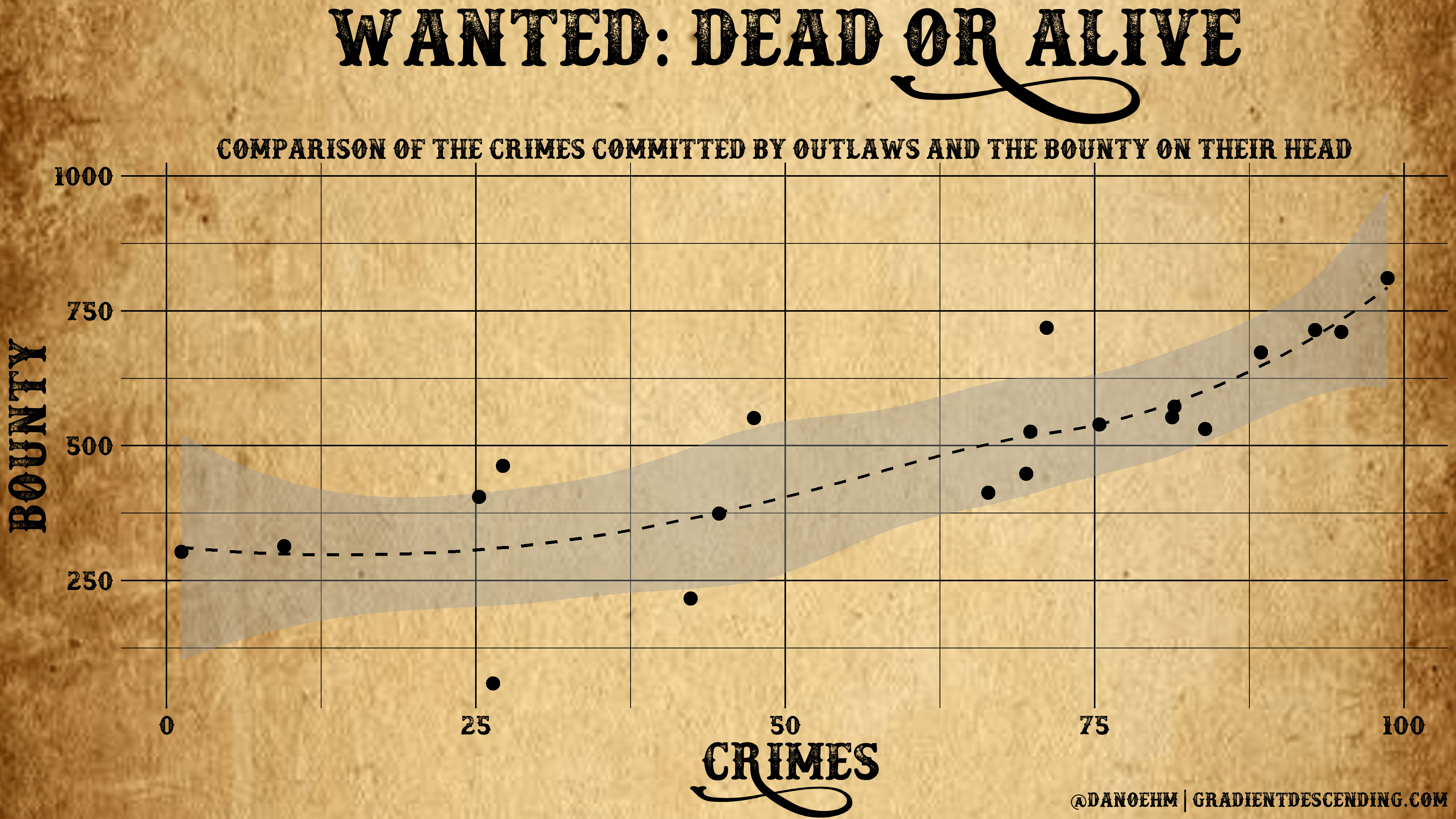
# wanted dead or alive
# generate data - unfortunately I couldn't find data on actual outlaws
n <- 20
x <- 100*runif(n)
y <- (25 + 0.005*x^2 + rnorm(n, 0, 10))*10
wanted <- data.frame(x, y) %>% 
  ggplot(aes(x = x, y = y)) +
  geom_smooth(col = "black", lty = 2) +
  geom_point(size = 4) +
  theme_minimal() +
  labs(title = "WANTED: DEAD OR ALIVE", 
       subtitle = "Relationship of the crimes committed by outlaws and the bounty on their head",
       x = "CRIMES", 
       y = "BOUNTY", 
       caption = "@danoehm | gradientdescending.com") + theme_minimal() +
  theme(
    text = element_text(family = "docktrin", size = 16*scale), 
    plot.title = element_text(size = 40*scale, hjust = 0.5),
    plot.subtitle = element_text(size = 14*scale, hjust = 0.5, margin = margin(t = 40)),
    plot.caption = element_text(size = 10*scale),
    legend.text = element_text(size = 12*scale),
    panel.grid = element_line(color = "black"),
    axis.title = element_text(size = 26*scale),
    axis.text = element_text(color = "black"))
png(file = ".s/wanted1.png", width = 3840, height = 2160, units = "px", res = 72*4)
ggdraw() +
  draw_image(".s/wanted_dead_or_alive_copped.png", scale = 1.62) + # a png of the background for the plot
  draw_plot(wanted)
dev.off()


# Horror movies
horror <- read_csv(".s/imdb.csv")
gghorror <- horror %>% 
  dplyr::filter(str_detect(keywords, "horror")) %>% 
  dplyr::select(original_title, release_date, vote_average) %>% 
  ggplot(aes(x = release_date, y = vote_average)) +
  geom_smooth(col = "#003300", lty = 2) +
  geom_point(size = 4, col = "white") +
  labs(title = "HORROR MOVIES!", 
       subtitle = "Average critics ratings of horror films and relationship over time",
       x = "YEAR", 
       y = "RATING", 
       caption = "Data from IMDB.\n@danoehm | gradientdescending.com") + theme_minimal() +
  theme(
    text = element_text(family = "swamp-witch", size = 16*scale, color = "#006600"), 
    plot.title = element_text(size = 48*scale, hjust = 0.5),
    plot.subtitle = element_text(family = "montserrat", size = 14*scale, hjust = 0.5, margin = margin(t = 30)),
    plot.caption = element_text(family = "montserrat", size = 8*scale),
    legend.text = element_text(size = 12*scale),
    panel.grid = element_line(color = "grey30"),
    axis.title = element_text(size = 26*scale),
    axis.title.y = element_text(margin = margin(r = 15)),
    axis.text = element_text(color = "#006600"),
    plot.background = element_rect(fill = "grey10"))
png(file = ".s/swamp.png", width = 3840, height = 2160, units = "px", res = 72*4)
gghorror
dev.off()

The post Adding Custom Fonts to ggplot in R appeared first on Daniel Oehm | Gradient Descending.