Cone plots (also known as 3-D quiver plots) represent vector fields defined in some region of the 3-D space.

A vector field associates to each point of coordinates (x, y, z) a vector of components (u, v, w).

In this post, we’ll explore how Plotly’s cone plots can be used to visualize atmospheric wind ?, magnetic fields, a trajectory of the Rössler System, and tangent vector fields to a surface.

So what’s a 3-D vector?

∙ A vector is a geometric object that has magnitude and direction.

∙ A 3-D vector is useful in any physical space where both magnitude and direction matter.

∙ In 3-D space, vectors are identified with triples of scalar components. In the case of the example image below: a = (ax, ay, az)

The direction of the vector field at a point is illustrated by a geometric cone, colored according to the vector norm (magnitude) at that point.

Cone plots can be used in a variety of abstract ways: to model a vortex (such as a tornado), illustrate an explicitly defined vector field, chart a hyperboloid, plot a system of non-linear ordinary differential equations, and show winds at various atmospheric levels.

For extra insights, check out our tutorial about making 3-D cone plots in Python with Plotly.

Cone Plot Showing Atmospheric Wind

This plot uses an explicitly defined vector field. A vector field refers to an assignment of a vector to each point in a subset of space.

In this plot, we visualize a collection of arrows that simply model the wind speed and direction at various levels of the atmosphere.

3-D weather plots can be useful to research scientists to gain a better understanding of the atmospheric profile, such as during the prediction of severe weather events like tornadoes and hurricanes.

Python code | Link to plot

Speaking of tornado-like rotations, here is an example of a cone plot of a vortex. The size of the cones are driven by wind speed.

Python code | Data | Link to plot

Cone Plot of a Magnetic Field

The Biot-Savart Law is an equation that describes the magnetic field created by a current-carrying wire.

It was named after Jean-Baptiste Biot and Felix Savart in 1820 when the pair derived the mathematical expression for magnetic flux density.

In this example, we leverage the law to create a hypothetical magnetic field created by an electric current moving through three circular loops.

Python code | Link to plot

Cone Plot Showing a Trajectory of the Rössler System

The Rössler system is a system of three ordinary differential equations, whose dynamics exhibits an attractor, or a set of states, invariant under the dynamics, towards which neighboring states in a given basin of attraction asymptotically approach in the course of dynamic evolution.

Originally studied by Otto Rössler, these differential equations “define a continuous-time dynamical system that exhibits chaotic dynamics associated with the fractal properties of the attractor.”

The equations have been found to be useful in modeling equilibrium in chemical reactions.

Python code | Link to plot

Cone Plot of a Tangent Vector Field

In mathematics, a tangent vector is a vector that is tangent to (or just touches) a curve or surface at a given point.

Tangent vector fields are an “essential ingredient in controlling appearance for applications ranging from anisotropic shading to texture synthesis and non-photorealistic rendering.”

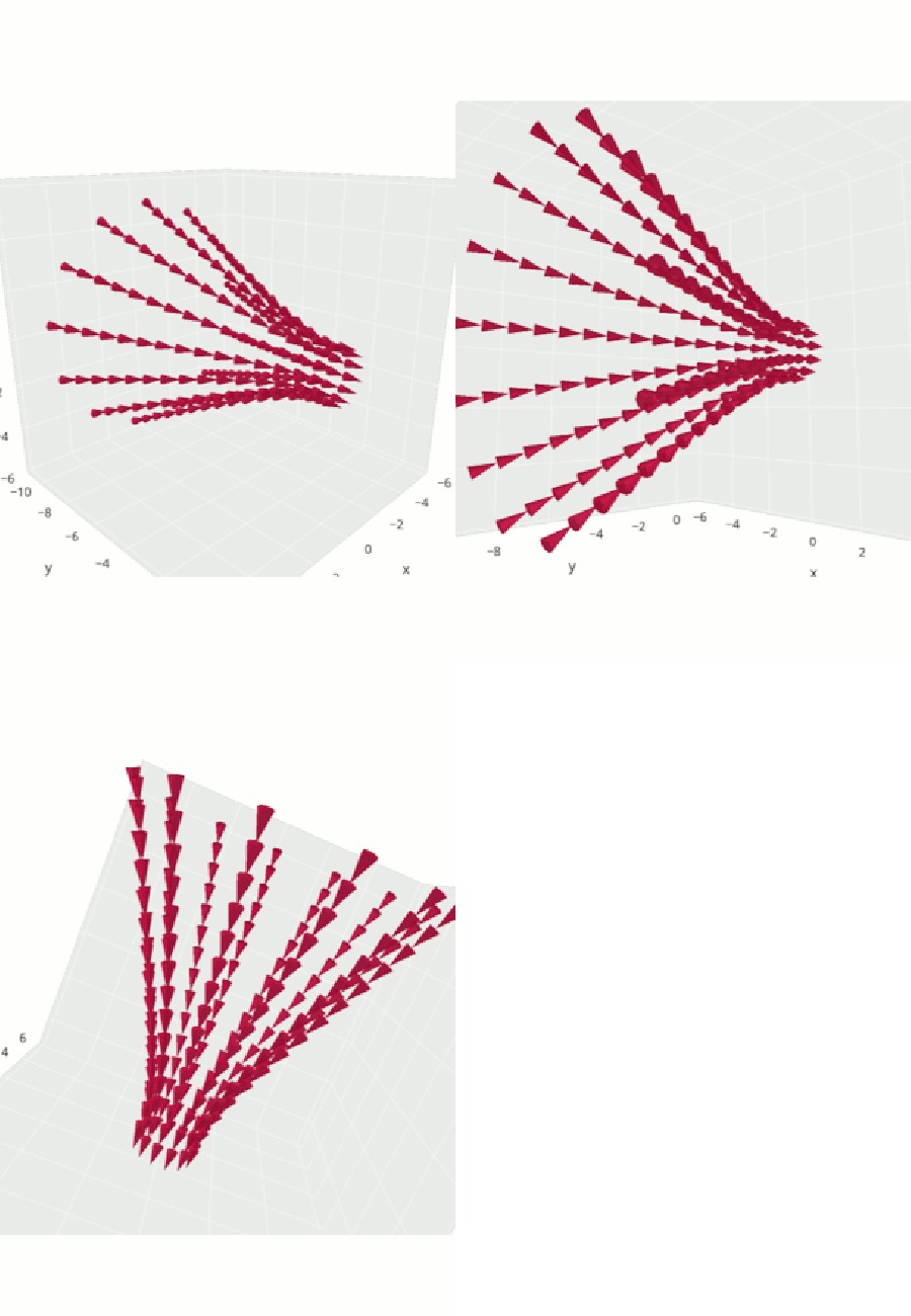
Below, we examine the tangent vector field along the coordinate lines of a parameterized hyperboloid.

Python code | Data | Link to plot

With 3-D cone plots in Plotly, you can allow the user to visualize vector fields across a variety of disciplines: meteorology, engineering, mathematics, and more. Bring your vectors to life with cone plots in Plotly!