Sub-Gaussian property for the Beta distribution (part 2)

Posted on December 20, 2017 by Julyan Arbel in Uncategorized | 0 Comments

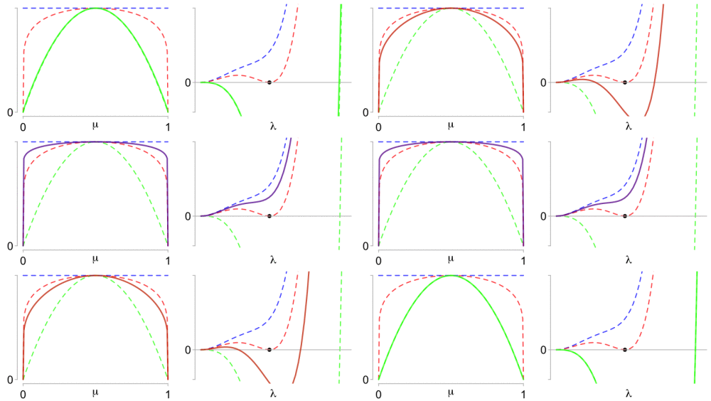
Left: What makes the Beta optimal proxy variance (red) so special? Right: The difference function has a double zero (black dot).

As a follow-up on my previous post on the sub-Gaussian property for the Beta distribution [1], I’ll give here a visual illustration of the proof.

A random variable $X$ with finite mean $\mu=\mathbb{E}[X]$ is sub-Gaussian if there is a positive number $\sigma$ such that:

$\mathbb{E}[\exp(\lambda (X-\mu))]\le\exp\left(\frac{\lambda^2\sigma^2}{2}\right)\,\,\text{for all } \lambda\in\mathbb{R}.$

We focus on X being a Beta $(\alpha,\beta)$ random variable. Its moment generating function $\mathbb{E}[\exp(\lambda X)]$ is known as the Kummer function, or confluent hypergeometric function $_1F_1(\alpha,\alpha+\beta,\lambda)$ . So X is $\sigma^2$ -sub-Gaussian as soon as the difference function

$u_\sigma(\lambda)=\exp\left(\frac{\alpha}{\alpha+\beta}\lambda+\frac{\sigma^2}{2}\lambda^2\right)-_1F_1(\alpha,\alpha+\beta,\lambda)$

remains positive on $\mathbb{R}$ . This difference function $u_\sigma(\cdot)$ is plotted on the right panel above for parameters $(\alpha,\beta)=(1,1.3)$ . In the plot, $\sigma^2$ is varying from green for the variance $\text{Var}[X]=\frac{\alpha\beta}{(\alpha+\beta)^2(\alpha+\beta+1)}$ (which is a lower bound to the optimal proxy variance) to blue for the value $\frac{1}{4(\alpha+\beta+1)}$ , a simple upper bound given by Elder (2016), [2]. The idea of the proof is simple: the optimal proxy-variance corresponds to the value of $\sigma^2$ for which $u_\sigma(\cdot)$ admits a double zero, as illustrated with the red curve (black dot). The left panel shows the curves with $\mu = \frac{\alpha}{\alpha+\beta}$ varying, interpolating from green for $\text{Var}[X]=\frac{\alpha\beta}{(\alpha+\beta)^2(\alpha+\beta+1)}$ to blue for $\frac{1}{4(\alpha+\beta+1)}$ , with only one curve qualifying as the optimal proxy variance in red.

References

[1] Marchal and Arbel (2017), On the sub-Gaussianity of the Beta and Dirichlet distributions. Electronic Communications in Probability, 22:1–14, 2017. Code on GitHub.
[2] Elder (2016), Bayesian Adaptive Data Analysis Guarantees from Subgaussianity, https://arxiv.org/abs/1611.00065