Abstract

The rwml-R Github repo is updated with R code for exploratory data analysis of New York City taxi data from Chapter 6 of the book “Real-World Machine Learning” by Henrik Brink, Joseph W. Richards, and Mark Fetherolf. Examples given include reading large data files with the fread function from data.table, joining data frames by multiple variables with inner_join, and plotting categorical and numerical data with ggplot2.

Data for NYC taxi example

The data files for the examples in Chapter 6 of the book are available at http://www.andresmh.com/nyctaxitrips/. They are compressed as a 7-Zip file archive (e.g. with p7zip), so you will need to have the 7z command available in your path to decompress and load the data. (On a mac, you can use Homebrew to install p7zip with the command brew install p7zip.)

Using fread (and dplyr…again)

As in Chapter 5, the fread function from the data.table library is used to quickly read in a sample of the rather large data files. It is similar to read.table but faster and more convenient. The following code reads in the first 50k lines of data from one of the trip data files and one of the fare data files. The mutate and filter functions from dplyr are used to clean up the data (e.g. remove data with unrealistic latitude and longitude values). The trip and fare data are combined with the inner_join function from the dplyr package.

tripFile1 <- "../data/trip_data_1.csv"
fareFile1 <- "../data/trip_fare_1.csv"
npoints <- 50000
tripData <- fread(tripFile1, nrows=npoints, stringsAsFactors = TRUE) %>%
  mutate(store_and_fwd_flag = 
           replace(store_and_fwd_flag, which(store_and_fwd_flag == ""), "N")) %>%
  filter(trip_distance > 0 & trip_time_in_secs > 0 & passenger_count > 0) %>%
  filter(pickup_longitude < -70 & pickup_longitude > -80) %>%
  filter(pickup_latitude > 0 & pickup_latitude < 41) %>%
  filter(dropoff_longitude < 0 & dropoff_latitude > 0)
tripData$store_and_fwd_flag <- factor(tripData$store_and_fwd_flag)
fareData <- fread(fareFile1, nrows=npoints, stringsAsFactors = TRUE)
dataJoined <- inner_join(tripData, fareData)
remove(fareData, tripData)

Exploring the data

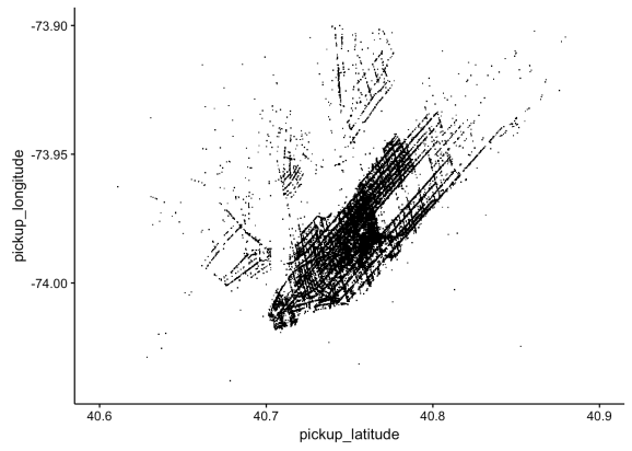
In the complete code-through, plots of categorical and numerical features of the data are made using ggplot2, including a visualization of the pickup locations in latitude and longitude space which is shown below. With slightly less than 50,000 data points, we can clearly see the street layout of downtown Manhatten. Many of the trips originate in the other boroughs of New York, too.

Feedback welcome

If you have any feedback on the rwml-R project, please leave a comment below or use the Tweet button. As with any of my projects, feel free to fork the rwml-R repo and submit a pull request if you wish to contribute. For convenience, I’ve created a project page for rwml-R with the generated HTML files from knitr, including a page with all of the event-modeling examples from chapter 6.

Download Fork