Let’s do something completely different today! I’m a huge data nerd and I’ve been uploading my music play information to a site called last.fm going back to 2005. Think of it like a “have read” book list for your music, except that it tracks every time you listen to a song.

I’ve collected quite a bit of data in the last 11 years so I decided to visualize my music habits in the last decade and see what I can learn about it.

For non-developers: If you’re not interested in coding just scroll past the code snippets and look at the nice plots and the accompanying explanation.

For developers: Check out the github repository for the project¹. Keep in mind that I assume you know how to code in R and are familiar with packages like dplyr, jsonlite, and ggplot2. If you’re not, this will not make sense and I suggest you start elsewhere.

Let’s go!

Getting the data

Unfortunately there’s no easy official method to download your entire dataset of scrobbles. One way or another you need to use the API to download your scrobbles one page at a time. You can either program against the API yourself or use somebody else’s code to pull the data into a CSV or another readable format.

Since I wanted to get at my data as quickly as possible, I went for the latter approach. After trying a couple of services I settled for a nice python script which you can get here.

Note: You might run into a site by Ben Benjamin which is more user-friendly, but keep in mind that it does not support UTF8 characters so it foreign characters like Korean, Japanese, and Chinese, will be messed garbled in your dataset.

The dataset

Once you’ve downloaded your scrobble data you’ll get a CSV file with a structure that looks close to this:

Column Name	Sample data
time	1327616201
song	Good Song
artist	Blur
album	Think Tank

Each row represents a single play of a track with the timestamp of the play, the name of the song, the artist, and the album to which the track belongs.

This information is taken from last.fm and not from the metadata tags of file to which you listened. This has implications for missing album data or unrecognized songs but more on that later.

If you used the python script to which I linked, you’ll have some additional ID strings like the MusicBrainz ID. Regardless of which method you chose, at a minimum you should have the data in the table above.

As for my dataset, I have a total of 29,674 scrobbles recorded between 13/02/2005 and 03/07/2016.

Loading the data

Let’s go ahead and load the data using the following code in a file called load.R²:

library(readr)
library(tibble)

col_names <- c(
   "date",
   "song",
   "artist",
   "album",
   "id1", "id2", "id3"
)

raw_scrobbles <- read_tsv("data-raw/raw_scrobbles.csv", col_names = col_names)
raw_scrobbles

The data I used was tab-separated so I used read_tsv, depending on your file you might want to use read_csv or any of the other read_* functions in the readr package. Look at the readr package documentation for more information.

Cleaning the data

There are two kinds of cleaning that need to happen and we'll tackle them in order:

1. Convert data to a useful format that makes analysis easier (Easy)
2. Fill in as much missing information as possible (Hard)

The date-time of the play is stored in the TSV file as seconds since the beginning of the epoch. I need to convert this into the more useful date-time type POSIXct to facilitate later manipulations. I also select the relevant columns, and the re-arrange by date.

library(dplyr)

tidy_scrobbles <- select(raw_scrobbles, date, song, artist, album)
tidy_scrobbles <- mutate(tidy_scrobbles, date = as.POSIXct(date, origin = "1970-01-01"))
tidy_scrobbles <- arrange(tidy_scrobbles, date)
tidy_scrobbles

This results in a tidy dataset that looks something like:

Source: local data frame [29,674 x 4]

                  date                    song            artist              album
                <time>                    <chr>           <chr>               <chr>
1  2005-02-13 12:20:00        Tired 'N' Lonely Roadrunner United                 NA
2  2005-02-13 12:20:01        Tired 'N' Lonely Roadrunner United                 NA
3  2005-02-13 12:20:02                  Suunta            Nicole Suljetut ajatukset
4  2005-02-13 12:20:03         Army Of The Sun Roadrunner United                 NA
5  2005-02-13 12:20:04         Army Of The Sun Roadrunner United                 NA
..                 ...                     ...               ...                ...

Well that was easy! But don't celebrate yet, because there's a clear problem. A bunch of tracks don't have album information. I'm not sure why the information is missing but it could potentially be a mismatch between the song name in the song metadata and last.fm's repository, the song is not part of an album, or the song is not in last.fm repository at all.

To figure out how much data is missing we need to first look at unique tracks and then count _NA_s in each column.

check_health <- function(data) {
  unique_tracks <- unique(select(data, -date))

  print(sum(is.na(unique_tracks$album)))
  print(sum(is.na(unique_tracks$artist)))
  print(sum(is.na(unique_tracks$song)))
}

check_health(tidy_scrobbles)

Luckily no artist or song names are missing, however 563 unique tracks are missing album information or just under 8% of the tracks. These account for ~7% of the total number of scrobbles. Let's see if we can fill some of this information automatically.

Using the Last.FM API to get album information

The last.fm API allows users to search for artists/songs and get information about artists, albums, and tracks.

The following query to method track.getInfo returns a JSON data structure with track information based on the artist and song name:

http://ws.audioscrobbler.com/2.0/?method=track.getInfo&artist=[ARTIST_NAME]&track=[TRACK_NAME]&api_key=[API_KEY]&format=json

The API key is obtained from the last.fm API page. Make sure to sign up for an account and checkout the documentation for the other parts of the API.

Let's write a function to build that query:

library(urltools)

build_track_info_query <- function(artist, track, api_key, base = "http://ws.audioscrobbler.com/2.0/") {
  base <- param_set(base, "method", "track.getInfo")
  base <- param_set(base, "artist", URLencode(artist))
  base <- param_set(base, "track", URLencode(track))
  base <- param_set(base, "api_key", api_key)
  base <- param_set(base, "format", "json")

  return(base)
}

The function takes an artist and song name, applies the URL encoding to the parameters, and builds the URL of the query³.

Next we fetch the JSON from the site and parse it for the relevant information. Here I use the jsonlite package to send the GET message and parse the response for the album name.

Since fetching JSON responses is a time consuming task, I use the package memoise to build result-caching versions of the fetching functions.

Finally, I create a new function that calls mapply to fetch the album information for a set of artists and song names.

library(jsonlite)
library(memoise)

fetch_track_album <- function(artist, track) {
  print(paste0("Fetching ", artist, " song: ", track))
  json <- fromJSON(build_track_info_query(artist, track))

  if (is.null(json$track$album)) return(NA)

  return(json$track$album$title)
}

memfetch_track_album <- memoise(fetch_track_album)

fetch_tracks_albums <- function(artists, tracks) {
  if (length(artists) != length(tracks)) {
    stop("Cannot fetch genres for songs because inputs are bad")
  }

  mapply(memfetch_track_album, artist = artists, track = tracks)
}

Now that we have a way to fetch the album name for multiple tracks we need a function to amend the missing album names to the original dataset.

fill_missing_albums <- function(data) {
  data %>%
    filter(is.na(album)) %>%
    distinct(song, artist, album) %>%
    mutate(album = fetch_tracks_albums(artist, song)) %>%
    left_join(data, ., by = c("artist", "song")) %>%
    transmute(date, artist, song, album = coalesce(album.x, album.y))
}

This worked pretty well but it didn't fill in all missing album names, nevertheless I decided to press on by saving out the clean dataset for the next phase.

Enriching data

To make things more interesting let's enrich the dataset with genre information. Last.fm doesn't assign genre information to songs and artists, instead relying on user-defined tags to provide that metadata. Let's fetch the most popular tags for each of the artists in the dataset and use that as the genre for all scrobbles⁴.

Since the procedure for building the query, getting the response, and parsing the JSON content is similar to fetching the album name. You can note the differences by looking at the functions, for building the query:

build_artist_toptags_query <- function(artist, api_key, base = "http://ws.audioscrobbler.com/2.0/") {
  base <- param_set(base, "method", "artist.gettoptags")
  base <- param_set(base, "artist", URLencode(artist))
  base <- param_set(base, "api_key", api_key)
  base <- param_set(base, "format", "json")

  return(base)
}

and fetching the JSON response and parsing it into a useful an R vector:

fetch_artist_toptags <- function(artist) {
  print(paste0("Fetching ", artist))
  json <- fromJSON(build_artist_toptags_query(artist))

  if (length(json$toptags$tag) == 0) return(NA)

  return(as.vector(json$toptags$tag[,"name"]))
}

Finally, make sure to save this tidy enriched data. We've done a lot of work so far, it would be a shame to lose it.

Let's get plotting!

To start with let's have a look at the overall number of plays per month to get a feel for the data.

library(dplyr)
library(ggplot2)
library(zoo)
library(hrbrmisc)

load("data/tidy_scrobbles_with_genres.RData")

# Wrapper around full_seq to work with zoo::yearmon objects
full_seq_yearmon <- function(x) {
  as.yearmon(full_seq(as.numeric(x), 1/12))
}

clean_scrobbles %>%
  count(yrmth = as.yearmon(date)) %>%
  complete(yrmth = full_seq_yearmon(yrmth)) %>%
  ggplot(aes(yrmth, n)) + geom_line() + geom_point() +
  scale_x_yearmon() +
  labs(x = "Month", y = "Plays", title = "Play counts per month",
       caption = "source: last.fm scrobbles") +
  theme_hrbrmstr()

To have a nice looking plot we summarize the counts per month with the help of as.yearmon in the zoo package and some dplyr goodness.

The dplyr::count function is a convenience function that wraps the often used _groupby, summarize, arrange pattern into a single function call. Here we create a new column called yrmth, group by it and then summarize the data frame by it.

If we were to plot this data now, ggplot2 would assume that the dataset is complete and create a single connected line across all the data points. We need to make sure that missing data is clearly visible on the plot, otherwise our visualizations are misleading. Let's pad the dataset with NA values (or 0 if you like) for the total count in months where no scrobbles happened.

We use full_seq in our own function full_seq_yearmon to generate a full sequence of yearmon objects from 2005 to 2016, and then invoke complete to expand the yrmth column to contain this sequence.

We use the hrbrmisc package by hrbrmstr because it contains some nice custom ggplot2 themes but it's completely optional.

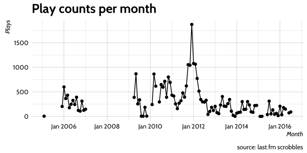
It seems a lot of data is missing, likely because scrobbling was not setup after a format or a reinstall of the music player.

There's also a large peak around January 2012; mid-way through my PhD. I'm not certain what caused the peak but I will take a look at this period in a follow up post.

Top 20 artists of all time

Let's look at the most popular aritsts overall.

top_artists <- clean_scrobbles %>%
  count(artist, genre, sort = T) %>%
  ungroup() %>%
  top_n(20)

First we count the number of scrobbles by artists, making sure to keep the genre column around, an then select the top 20 artists.

The next part is specific to my dataset, but I had to translate the names of Korean and Japanese bands into English since I couldn't get ggplot2 to display the characters correctly. We'll be translating these artists names again so we have a function to make that easier.

translate_artists <- function(x) {
  recode(
    artist,
    소녀시대`  = "Girls' Generation",
    `HOME MADE 家族` = "HOME MADE KAZOKU"
  )
}

top_artists_translate <- top_artists %>%
  mutate(artist = translate_artists(artist))

And finally we create a lollipop-esque plot of the artists ranked by play counts, colored by the genre:

top_artists_translate %>%
  ggplot(aes(reorder(artist, n), n, color = genre)) +
   geom_segment(aes(xend = reorder(artist, n)), yend = 0, color = 'grey50') +
     geom_point(size = 3) +
  coord_flip() +
  labs(y = "Plays", x = "", title = "My taste is all over the place", subtitle = "Top 20 Artist by plays", caption = "source: last.fm scrobbles") +
  theme_hrbrmstr() +
  scale_color_viridis(discrete = T, name = "Genre") +
  theme(panel.grid.major.x = element_blank(),
        panel.grid.minor.x = element_blank(),
        panel.grid.major.y = element_line(color = 'grey60', linetype = 'dashed'))

The code above then produces the following ranking plot:

   

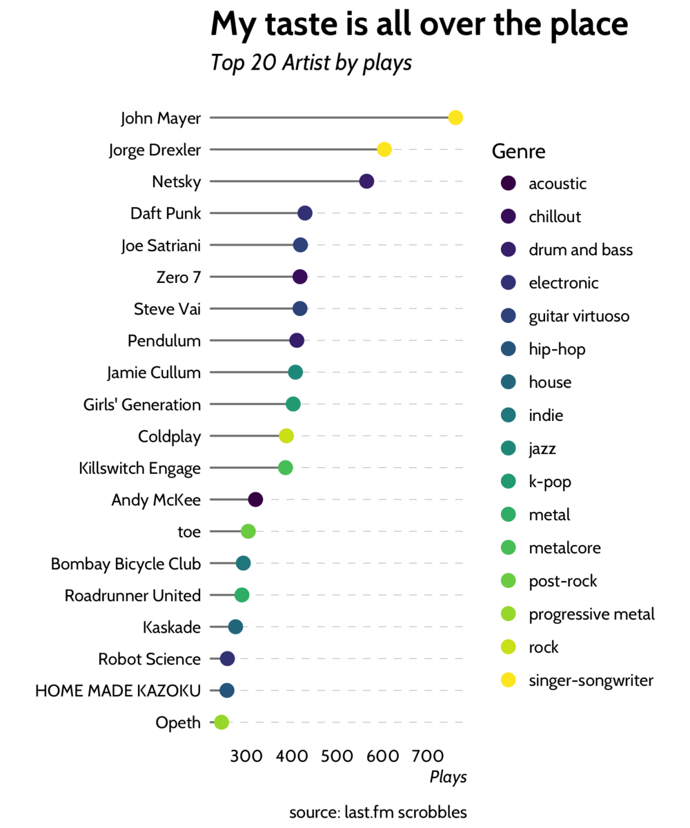
Turns out I'm a big fan of John Mayer and in general my taste in music is very varied.

Artists preference over time

Let's take a look at how artist preference evolves from year to year, with some inspiration from this beautiful subway-style plot that we've adapted to our needs:

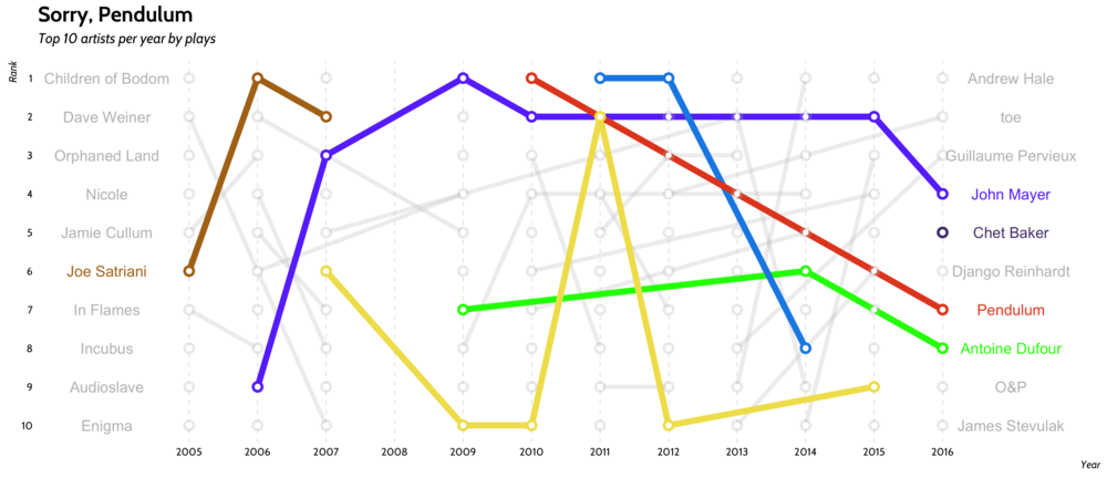
That's really nice isn't it? For some reason the popularity of Pendulum has been steadily decreasing, while John Mayer has remained pretty steady.

Let's take a look at how we made that plot. First we need to count the number of plays per year per artists and select only the top 10 artists per year and then rank the results using row_number. We use row_number to avoid having multiple artists with the same rank as they will overlap in the final plot:

# Lubridate For the year function
library(lubridate)

tops <- 10

artist_ranking <- clean_scrobbles %>%
  mutate(artist = translate_artist(artist)) %>%
  count(year = year(date), artist) %>%
  group_by(year) %>%
  mutate(rank = row_number(-n)) %>%
  filter(rank < tops + 1)

To make the plot we start by building data frames that contain the names of the top artists at the either end of the plot:

artist_end_tags <- artist_ranking %>%
  ungroup() %>%
  filter(year == max(year)) %>%
  mutate(year = as.numeric(year) + 0.25)

artist_start_tags <- artist_ranking %>%
  ungroup() %>%
  filter(year == min(year)) %>%
  mutate(year = as.numeric(year) - 0.25)

These data frames will be used to define the labels on the left and right of the plot, so we increment/decrement the year to avoid overlapping with the edges of the plot.

To make the plot clearer I highlight a few artists by assigning them a color, and set the other artists to gray so they blend nicely with the background:

colors <- c("John Mayer" = "#6a40fd", "Netsky" = "#198ce7", "Chet Baker" = "#563d7c", "Jorge Drexler" = "#f1e05a",
            "Joe Satriani" = "#b07219", "Pendulum" = "#e44b23", "Antoine Dufour" = "green")

othertags <- artist_ranking %>% distinct(artist) %>% filter(!artist %in% names(colors)) %>% .$artist

colors <- c(colors, setNames(rep("gray", length(othertags)), othertags))

highlights <- filter(artist_ranking, artist %in% names(colors)[colors != "gray"])

Finally we put it all together

ggplot(data = artist_ranking, aes(year, rank, color = artist, group = artist, label = artist)) +
  geom_line(size = 1.7, alpha = 0.25) +
  geom_line(size = 2.5, data = highlights) +
  geom_point(size = 4, alpha = 0.25) +
  geom_point(size = 4, data = highlights) +
  geom_point(size = 1.75, color = "white") +
  geom_text(data = artist_start_tags, x = 2003.8, size = 4.5) +
  geom_text(data = artist_end_tags, x = 2017, size = 4.5) +
  scale_y_reverse(breaks = 1:tops) +
  scale_x_continuous(
    breaks = seq(min(artist_ranking$year), max(artist_ranking$year)),
    limits = c(min(artist_ranking$year) - 1.5, max(artist_ranking$year) + 1.6)) +
  scale_color_manual(values = colors) +
  theme_hrbrmstr() + theme(
    legend.position = "",
    panel.grid.major.y = element_blank(),
    panel.grid.minor.y = element_blank(),
    panel.grid.minor.x = element_blank(),
    panel.grid.major.x = element_line(color = 'grey60', linetype = 'dashed')) +
  labs(x = "Year", y = "Rank", title = "Sorry, Pendulum",
       subtitle = "Top 10 artists per year by plays")

Note that we increase the limits on the X axis beyond the range of the data to make the artist labels at the start and end visible.

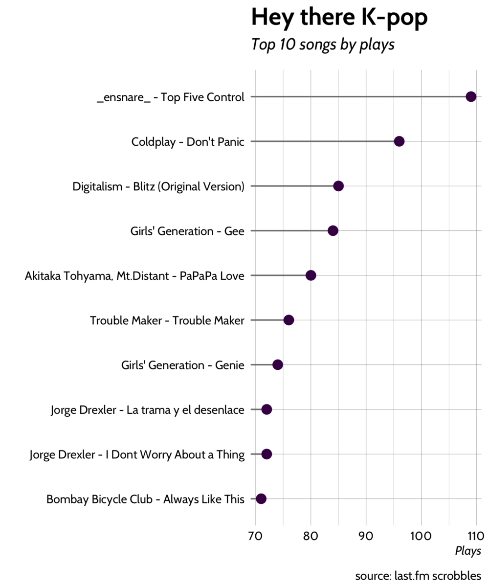
Top 10 songs

Next let's look at the top 10 songs, the process is similar to making the artist ranking plot. Here we need to translate the names of foreign songs as well, and then we use unite to create nice labels for the plot that include the artist and song name.

tops <- 10

translate_songs <- function(x) {
  recode(
    x,
    `소녀시대 (girls' generation)` = "Girls' Generation",
    `소원을 말해봐 (genie)` = "Genie"
  )
}

top_songs <– clean_scrobbles %>%
  count(song, artist, sort = T) %>%
  ungroup() %>%
  top_n(tops) %>%
  mutate(
    artist = translate_artists(artist),
    song = translate_songs(song)
  ) %>%
  unite(fullname, artist, song, sep = " - ", remove = F)

top_songs %>%
  ggplot(aes(reorder(fullname, n), n)) +
  geom_segment(aes(xend = reorder(fullname, n)), yend = 0, color = 'grey50') +
  geom_point(size = 3, color = viridis(1)) +
  scale_color_viridis() + coord_flip() + theme_hrbrmstr() + theme(legend.position = "") +
  labs(x = "", y = "Plays", title = "Hey there K-pop", subtitle = "Top 10 songs by plays",
       caption = "source: last.fm scrobbles")

It seems that John Mayer holds the top spot because I listed to many of his songs as smaller number of times. As a result none of his songs cracked the top 10. On the other hand it's interesting that 3 out of the top 10 songs are K-pop songs.

   

Genres over time

Let's make another subway-style ranking plot for the top 10 genres. The code is similar to that which created the artists ranking plot, so I omit it here.

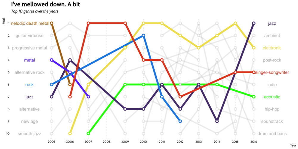
It seems my love for all forms of metal has decreased towards the end of my high-school years, with acoustic, singer-songwriter, electronic, and jazz music picking up the mantel. Over time my taste in music has mellowed a bit.

One more thing

This was a very fun project, and I learnt a bunch about API usage and how to make more complicated visualizations with ggplot2. I'm excited to do this again in another 10 years and see how my taste has changed from today.

As a fun take away for you the reader I've created a Spotify playlist with some of my top songs of all time:

Top Songs by Jay Blanco

Until next Time. Have a great one.

-- Jay Blanco

For great R and data analytics content please checkout R-Bloggers.

Footnotes

1. The code is not production quality, but feel free to adapt it. ↩
2. I used throw-away labels for the ID columns cause I'm not keeping them. ↩
3. I realize that the httr package might be a more modern approach that using urltools, but frankly I didn't do much API work before this. ↩
4. This is certainly not perfect, but we are aiming for good enough. Saving tags for all songs would take too long. ↩