Since summer is coming and meaning vacations we are going to explore the tourism in France. To do so, we are going to explore the number of hotel room per deparements (a small administrative area in France) and see if somes show more tourist appeal than others.

1.The data:

To do this analysis, we are gong to use several dataset availables online:

• INSEE: Ranked hotel in France by Zip Code (DF1)
• INSEE: Link between zip code, and admnistrative area (DF2)
• INSEE: Population per administrative area (DF3)
• Key table to join area name and number (DF4)
• Highchart: A map of France at the proper administrative level

1.b: Packages:
library(data.table)
library(highcharter)
library(rgeos)
library(rgadal)
library(ggplot2)
library(viridis)

2.Data preprocessing:

We wish to assess the number of hotel room per capita in the different area, so w will:

1. Count the number of rooms per ZIP-code using DF1:

##Loading the number of room per ZIP code
HotelFrance=data.table(read.csv("~/data/DF1.csv", sep=";", stringsAsFactors=FALSE))
HotelFrance
HotelAgg=HotelFrance[,.(Lits=sum(as.numeric(NOMBRE.DE.CHAMBRES,na.rm=T))),by=CODE.POSTAL]
HotelAgg=HotelAgg[!is.na(Lits)]
setkey(HotelAgg,CODE.POSTAL)

2.Join the ZIP code with the area using DF2

##Join between Zip code/area code and number of rooms
##Jointure
CPInsee <- read.csv("~/data/DF2.csv", sep=";", stringsAsFactors=FALSE)
CPInsee<-data.table(CPInsee)
Jointure=data.table(CPInsee[,.(CODE.POSTAL=as.numeric(Code.Postal),Dep=Code.DÃ.partement)])
DT<-unique(merge(HotelAgg,Jointure,by='CODE.POSTAL'))
DT[,id:=as.character(Dep)]
DT=DT[,.(Lits=sum(Lits)),by=id]

3. Loading the departement names (DF4) and correcting some typos:

##Loading the number of room per ZIP code
##Join between Zip code/area code and number of rooms
##Jointure
CPInsee=read.csv('~/Data/DF3.csv', sep=';', stringsAsFactors=FALSE)
CPInsee=data.table(CPInsee)
Jointure=data.table(CPInsee[,.(CODE.POSTAL=as.numeric(Code.Postal),Dep=Code.DÃ.partement)])
DT=unique(merge(HotelAgg,Jointure,by='CODE.POSTAL'))
DT[,id:=as.character(Dep)]
DT=DT[,.(Lits=sum(Lits)),by=id]

4.Joining the population data and the Datatable from 3.

###Exploring the number of room per capita:

##Loadin the number of capita per departement
PopDep <- data.table(read.csv("~/Data/DF3.csv", sep=";",stringsAsFactors = F))
PopDep[,Population:=as.numeric(gsub(' ','',Population))]

###Joint between population/room
DTroom<-merge(DT,departement,by.x='id',by.y='V2',all.x=T)
DTwithPop<-data.table(merge(DTroom,PopDep,by.x='id',by.y='Dep'))

3. A first plot

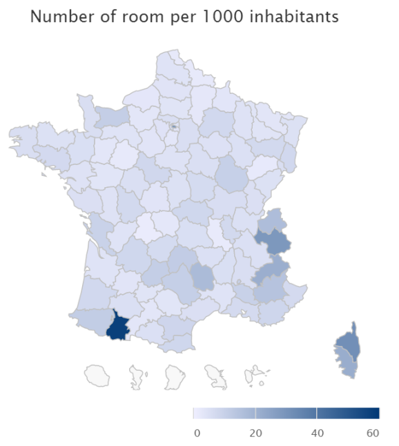
Now that all our data are together, let’s plot a first map: The number of rooms per 1000 inhabitants:

###Correcting some mistakes
DTwithPop[id=='2A',V3:='Haute-Corse']
DTwithPop[id=='2B',V3:='Corse-du-Sud']
DTwithPopPlot<-DTwithPop[,.(Dep=V3,RoomCapita=round(Lits/Population*1000,1))]

Map<-"fr-all-all.geo.json" %>%
jsonlite::fromJSON(simplifyVector = FALSE)
highchart(type = "map") %>%
hc_title(text = "Number of room per 1000 inhabitants") %>%
hc_add_serie_map(world,DTwithPopPlot,'RoomCapita',c('name','Dep'))%>%
hc_mapNavigation( enableMouseWheelZoom=T)

We corrected some names to have Corsica correctly plotted. Running the code above, you should get the same plot plot, but it will be interactive.

4. A first model:

As we see above, most of the areas have the same colors, meaning we should be able to fit a linear model Number Of Room~Number Of Inhabitants.

###In an ideal case, the number of room should be proportionate to the number of inhabitants
Model1=lm(data=DTwithPop,Lits~Population)
Model2=lm(data=DTwithPop[V3!='Paris'],Lits~Population)
summary(Model1)
summary(Model2)
##R²=0.28, not that bad and 0.36 without paris
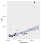
ggplot(data=DTwithPop,aes(x=Population,y=Lits))+geom_point()+geom_smooth(method='lm')+xlab('Inhabitants')+ylab('Room')
ggplot(data=DTwithPop[V3!='Paris'],aes(x=Population,y=Lits))+geom_point()+geom_smooth(method='lm')+xlab('Inhabitants')+ylab('Room')

Using this code, we are getting an R² of 0.28 for Model1 and 0.37 for the second model. Deleting Paris from the model seems appropriate for several reasons:

• It’s a clear outlier with an internally deleted residuals of 21 (!) and a cook’s D of 4.1.
• The outlyingness can easily be explained by the fact that Paris is … well Paris and attract much more tourist than most of France. Paris should be studied on its own.

The study will now focus on the second model.

5. A geographic exploration of the residuals of Model 2

Our goal here isn’t that much the model but seeing how the differents area behave according to the model. Instead of plotting the residuals distribution, let’s see how the maps of France look when each departement is assigned its resiudal value. A strongly negative residual would show a low appeal (i.e a lot of inhabitants but only a few tourists facilities) whereas a highly positive residual would show a high appeal.

##If the data was to be fitted by a lm, all the area should have more or less the sam color.
##Some outliers, Paris, Corsica, HAute Pyréne and Alps
n <- 6
dstops <- data.frame(q = 0:n/n, c = substring(brewer.pal(n+1, 'RdBu'), 0, 7))
dstops <- list.parse2(dstops)

GeoResidual2<-data.table(Dep=DTwithPopPlot[Dep!='Paris',Dep],Res=Model2$residuals)
MapResiduals2<-"fr-all-all.geo.json" %>%
jsonlite::fromJSON(simplifyVector = FALSE)
highchart(type = "map") %>%
hc_title(text = "Residuals per area") %>%
hc_add_serie_map(world,GeoResidual2,'Res',c('name','Dep'))%>%
hc_mapNavigation( enableMouseWheelZoom=T)%>%
hc_colorAxis(min = -10000, max =10000,stops = dstops)

After some investigations, the map seems logical:

• The deep blue area with a strong tourist attraction are respectively (from west to east): Pyrenees, French riviera, the Alps and Corsica.
  Pyrenees and the Alps have both a lot of ski resort and aren’t densely populated.
  French rivieria is more populated which lower the impacts of its tourism.
• The north of France is densely populated and hasn’t a lot of tourist appeal.