twilight zone [of statistics]
Want to share your content on R-bloggers? click here if you have a blog, or here if you don't.
“I have decided that mixtures, like tequila, are inherently evil and should be avoided at all costs.” L. Wasserman
Larry Wasserman once remarked that finite mixtures were like the twilight zone of statistics, thanks to the numerous idiosyncrasies associated with such models. And George Casella had similar strong reservations about mixture estimation. Avi Feller and co-authors [including Natesh Pillai] have just arXived a paper on this topic, exhibiting shocking (!) properties of the MLE! Their core example is a mixture of two normal distributions with known common variance and known weight different from 0.5, which ensures identifiability. This is a favourite example of mine that we used for instance in our book Introducing Monte Carlo methods with R. If only because we can plot the likelihood and posterior surfaces. (Warning: I wrote those notes on an earlier version of the paper, so mileage may vary in terms of accuracy!)
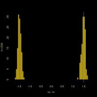
![repartition of the MLE of Δ when Δ=0.75σ [left] and when Δ=0.25σ [right] (c.) Feller et al., 2006](https://xianblog.files.wordpress.com/2016/02/wronmix.jpg?w=450&resize=450%2C168#038;h=168) The “shocking” discovery in the paper is that the MLE is wrong as often as not in selecting the sign of the difference Δ between both means, with an additional accumulation point at zero. The global mode may thus be in the wrong place for small enough sample sizes. And even for larger sizes: when the difference between the means is small the likelihood is likely to be unimodal with a mode quite close to zero. (An interesting remark is that the likelihood derivative is always zero at Δ=0 when considering the special case of both means equal to -Δ and to πΔ/(1-π), respectively, which implies that the overall mean of the mixture is equal to zero. A potential connection with our reparameterisation paper, maybe?)
The “shocking” discovery in the paper is that the MLE is wrong as often as not in selecting the sign of the difference Δ between both means, with an additional accumulation point at zero. The global mode may thus be in the wrong place for small enough sample sizes. And even for larger sizes: when the difference between the means is small the likelihood is likely to be unimodal with a mode quite close to zero. (An interesting remark is that the likelihood derivative is always zero at Δ=0 when considering the special case of both means equal to -Δ and to πΔ/(1-π), respectively, which implies that the overall mean of the mixture is equal to zero. A potential connection with our reparameterisation paper, maybe?)
The alternative proposed by Avi and his co-authors is to proceed through moments, i.e., to revert to Pearson (1892). There are however difficulties with this approach, first and foremost the non-uniqueness of the moment equations used to estimate Δ. For instance, the second cumulant equation chosen by the authors is not always defined as opposed to the third cumulant equation (why not using this third cumulant then). Which does not always produce the right sign… But, in a strange twist, the authors turn those deficiencies into signals for both pathologies (wrong sign and “pile-up” at zero).
“…the grid bootstrap yields an exact p-value for any valid test statistic.”
The most importance issue in this framework being in estimating the parameters, the authors opt for an approach based on tests, which is definitely surprising given the well-known deficiencies of standard tests in mixtures. The test chosen here is a Wald test with a statistic equal to the χ² version of the first cumulant differences. I am surprised that the χ² approximation works in such an unfriendly setting. And I do not understand how the grid is used, unless a certain degree of approximation is accepted, which takes us back to the “dark ages” of imposing a minimal distance Δ to achieve consistency, as in Ghosh and Sen (1985).
“..our concern about sign error is trivial in the Bayesian setting: the global mode is simply a poor summary of a multi-modal posterior. More broadly, the weak identification issues we highlight in this paper are not necessarily relevant to a strict Bayesian.”
A priori, I do not think pathologies of the MLE always transfer to Bayes estimators, unless one uses the MAP as an [poor] estimator. But using the MAP is not necessary since posterior means are meaningful in this identified setting, where label switching should not occur. However, running the same experiments with a Gaussian prior on both means and using the posterior mean as my estimator, I did obtain the same pathology of Bayes estimates [also produced in the supplementary material] not concentrating on the true value of the difference, but putting weight on the opposite value and at zero. Using a less standard prior inspired by David Rossell’s talk on non-local priors two weeks ago, which avoids a neighbourhood of zero, I did not get a much different picture as illustrated below:
Overall, I remain somewhat uncertain as to what to conclude from this pathological behaviour. When both means are close enough, the sign of the difference is often estimated wrongly. But that could simply mean that the means are not significantly different, for that sample size…
Filed under: Books, pictures, R, Statistics, University life Tagged: Bayesian estimation, convergence of Gibbs samplers, Gibbs sampling, identifiability, label switching, method of moments, Metropolis-Hastings algorithm, mixtures of distributions, MLE, multimodality, non-local priors
R-bloggers.com offers daily e-mail updates about R news and tutorials about learning R and many other topics. Click here if you're looking to post or find an R/data-science job.
Want to share your content on R-bloggers? click here if you have a blog, or here if you don't.


