The PM 2.5 checker written by R has been working nicely for me.  I put a shortcut icon of this small script on my desktop PC, to check the air pollution when I run.  The Ibaraki Prefecture Agency has been increasing watching points for PM 2.5 concentration from China.  A problem is that I cannot picture to myself all the observation locations exactly.

Fig. 1a. March 2013

Fig. 1b. January 2016

Now, time to use the power of GIS.

1. Shape file

City boundary data is published by Japanese government agency at http://www.gsi.go.jp/kankyochiri/gm_jpn.html and http://www.gsi.go.jp/kankyochiri/gm_japan_e.html (English).

1. Download gm-jpn-all_u_2_1.zip (8MB) , which is the current (2015, v.2.1) file with all layers.
2. Unzip to ~/var/gis/gm-jpn-all_u_2_1, or somewhere you like.
3. The city boundary shape file is polbnda_jpn.shp.

Let’s see if this map data works or not.

Here I use CRAN package maptools.

library(maptools)
cities.japan <- 
    readShapeSpatial('~/var/gis/gm-jpn-all_u_2_1/polbnda_jpn.shp')
plot(cities.japan)

A map of Japan is drawn. It’s working.

Fig. 2. City boundaries in Japan

I don’t need the entire Japan but Ibaraki Ken local area only.

cities.ibaraki <- 
    cities.japan[cities.japan$nam == 'Ibaraki Ken',]
plot(cities.ibaraki)

It’s perfect!  The specification of data can be found at http://www.iscgm.org/gm/spec.html.

Fig. 2. City boundaries in Ibaraki

This map is plotted with Longitude on X-axis and with Latitude on Y-axis.  The range can be shown by @bbox.

> cities.ibaraki@bbox
min       max
x 139.6879 140.85190
y  35.7396  36.94547

These values are useful to overwrite multiple layers on the same plot. Let’s see the following plot fits exactly on the previous one.

plot(cities.ibaraki, add=T, 
     xlim=cities.ibaraki@bbox['x',], 
     ylim=cities.ibaraki@bbox['y',], 
     border=rgb(1,0,0,0.2), lwd=8)

Plot method is expanded for the class SpatialPolygons, and specific parameters can be found at the help page of SpatialPolygons-class.

Finally, I’m ready to add a data point.

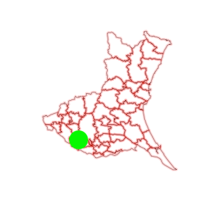
points(140, 36, col='green', cex=8, pch=19)

A green circle is drawn at (140°E, 36°N).  My first GIS plot is successfully done.

Fig. 4. Green circle (140°E, 36°N) on Ibaraki map

2. KML file

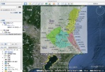
Unfortunately, the agency page doesn’t show the exact location of the observatories.  They are just shown on the map without geographical data.  So I have to generate longitude and latitude pairs for every observation points.  Using the Google Earth is a good way to generate such a location data interactively.

1. Add the agency map picture as a transparent image overlay on the Google Earth.
2. Adjust the size and position of the image overlay to fit the google map.
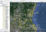
3. Add point markers at the observatories.  With appropriate names to merge the PM 2.5 data.  Id (局番) and name (測定局) will be good choices.
4. Save as a KML file, or KMZ file.

Fig. 5a. adjusting image overlay

Fig. 5b. image overlay fits

Fig. 5c. marking points

Fig. 5d. almost done

Fig. 5e. done

Placemark tags in the KML file denote the points marked. The Point/coordinates element has the location of a mark (longitude, latitude, height).

<Placemark>
    <name>101 北茨城中郷</name>
    <LookAt>
        <longitude>140.7467127432552</longitude>
        <latitude>36.78449028668253</latitude>
        <altitude>0</altitude>
        <heading>0</heading>
        <tilt>0</tilt>
        <range>999.4150061410331</range>
        <gx:altitudeMode>relativeToSeaFloor</gx:altitudeMode>
    </LookAt>
    <styleUrl>#m_ylw-pushpin</styleUrl>
    <Point>
        <gx:drawOrder>1</gx:drawOrder>
        <coordinates>140.7467127432552,36.78449028668252,0</coordinates>
    </Point>
</Placemark>

Let’s extract these data from the KML file (obs.ibaraki.kml) as an XML.

library(XML)
observatories <- xmlInternalTreeParse('~/var/obs.ibaraki.kml')

A command, xpathSApply(observatories, '//kml:Placemark'), extracts a list of Placemark elements from the entire KML tree.  Simultaneously, it can parse inside the Placemark with a function that evaluates each node.

parsePlacemarks <- function(node) {
  x <- xmlToList(node)
  c(splitNameId(x[['name']]), 
    splitLongLat(x[['Point']][['coordinates']]))
}

splitNameId <- function(x) {
  # fixed delimiter located at 4
  at <- 4
  id <- substring(x, 1, at - 1)
  name <- substring(x, at + 1)
  c(id=id, name=name)
}

splitLongLat <- function(x) {
  # three values are delimited by a comma
  coordinates <- strsplit(x, ',')[[1]]
  c(longitude=coordinates[1], latitude=coordinates[2])
}

placemarks <- xpathSApply(observatories, 
              '//kml:Placemark', parsePlacemarks)

It is a simple matrix that has data required, but all the element types are characters.

> str(placemarks)
 chr [1:4, 1:42] "101" "北茨城中郷" "140.7467127432552" ...
 - attr(*, "dimnames")=List of 2
  ..$ : chr [1:4] "id" "name" "longitude" "latitude"
  ..$ : NULL

> placemarks
          [,1]                [,2]                [,3]               
id        "101"               "102"               "103"              
name      "北茨城中郷"        "高萩本町"          "日立市役所"       
longitude "140.7467127432552" "140.7187301610473" "140.6518222207606"
latitude  "36.78449028668252" "36.71661395294382" "36.59936944459775"
          [,4]                [,5]                [,6]               
id        "104"               "106"               "107"              
name      "日立会瀬"          "日立多賀"          "常陸那珂勝田"     
longitude "140.6590441019378" "140.6283284820888" "140.5346855578042"
latitude  "36.57999478775783" "36.5549260221179"  "36.39667064061915"
---
more 36 columns

Finally, convert it to a data frame.

placedata <- data.frame(id=placemarks['id',], 
  obs.name=placemarks['name',], 
  longitude=as.numeric(placemarks['longitude',]), 
  latitude=as.numeric(placemarks['latitude',]))

> str(placedata)
'data.frame':    42 obs. of  4 variables:
 $ id       : Factor w/ 42 levels "101","102","103",..: 1 2 3 4 5 6 7 8 9 10 ...
 $ obs.name : Factor w/ 42 levels "つくば高野","ひたちなか",..: 41 8 35 34 37 17 23 27 4 18 ...
 $ longitude: num  141 141 141 141 141 ...
 $ latitude : num  36.8 36.7 36.6 36.6 36.6 ...

> head(placedata)
   id     obs.name longitude latitude
1 101   北茨城中郷  140.7467 36.78449
2 102     高萩本町  140.7187 36.71661
3 103   日立市役所  140.6518 36.59937
4 104     日立会瀬  140.6590 36.57999
5 106     日立多賀  140.6283 36.55493
6 107 常陸那珂勝田  140.5347 36.39667

3. Merge data and location together

The previous PM 2.5 script must be modified slightly to have an id column as a key on merging.

air.ibaraki <- readHTMLTable('http://www.taiki.pref.ibaraki.jp/data.asp', 
  which=6, skip.rows=1, trim=T, 
  colClasses=c('integer', 'character', rep('numeric', 13)))

pm.2.5.ibaraki <- air.ibaraki[!is.na(air.ibaraki[,12]), c(1,2,12)]
names(pm.2.5.ibaraki) <- c('id', 'name', 'pm2.5')
for(i in 1:2)
  pm.2.5.ibaraki[,i] <- as.factor(as.character(pm.2.5.ibaraki[,i]))

Merge by id and get an inner join:

pm25 <- merge(pm.2.5.ibaraki, placedata, by='id')

Merge by id and get a left outer join:

pm25.all <- merge(pm.2.5.ibaraki, placedata, by='id', all.x=T)

Check if all the data have locations:

pm25.noplace <- pm25.all[is.na(pm25.all[,'obs.name']),]

> nrow(pm25.noplace)
[1] 0

Successfully merged.

> head(pm25)
   id       name pm2.5   obs.name longitude latitude
1 101 北茨城中郷     0 北茨城中郷  140.7467 36.78449
2 103 日立市役所     6 日立市役所  140.6518 36.59937
3 106   日立多賀     1   日立多賀  140.6283 36.55493
4 110   大宮野中     5   大宮野中  140.4109 36.54277
5 111 笠間市役所     7 笠間市役所  140.2375 36.38522
6 121 鉾田保健所     2 鉾田保健所  140.5167 36.15960

4. Plot

The most important point of GIS plotting is how the data values are presented on the map.  In this time, I use both of color and bubble size to show the PM 2.5 concentration.

The following function will give a good size of points.

to.cex <- function(x) {
  ifelse(x > 5, x/10, 0.5)
}

Because the data sometimes has a minus (maybe an error) value, a constant size (0.5) is applied to the values under 5 μg/m³.  For clear viewing, I want use only three colros, namely, green, yellow and red.

• Values under 30 μg/m³ are green; means safe.
• Values between 30 and 60 μg/m³ are yellow; means warn.
• Values over 60 μg/m³ are red; means danger.

to.col <- function(x) {
  x.3 <- ifelse(x < 30, 1, ifelse(x < 60, 2, 3)) 
  c('forestgreen', 'darkorange', 'deeppink')[x.3]
}

Finally, plot points on the map.

plot(cities.ibaraki, border='gray')
with(pm25, text(x=longitude, y=latitude, labels=name, 
                col='royalblue', pos=1, cex=0.7))
points(latitude ~ longitude, pm25, 
       cex=to.cex(pm2.5), col=to.col(pm2.5))

Fig. 6. PM 2.5 chart with GIS

5. Sources

• Available at GitHub.
• Download zip or tar.gz archive.
• View the KML file of Ibaraki air observatories.