Image Credit: Doug Buckley of http://hyperactive.to

There are many different techniques that be used to model physical, social, economic, and conceptual systems. The purpose of this post is to show how the Kermack-McKendrick (1927) formulation of the SIR Model for studying disease epidemics (where S stands for Susceptible, I stands for Infected, and R for Recovered) can be easily implemented in R as a discrete time Markov Chain using the markovchain package.

A Discrete Time Markov Chain (DTMC) is a model for a random process where one or more entities can change state between distinct timesteps. For example, in SIR, people can be labeled as Susceptible (haven’t gotten a disease yet, but aren’t immune), Infected (they’ve got the disease right now), or Recovered (they’ve had the disease, but no longer have it, and can’t get it because they have become immune). If they get the disease, they change states from Susceptible to Infected. If they get well, they change states from Infected to Recovered. It’s impossible to change states between Susceptible and Recovered, without first going through the Infected state. It’s totally possible to stay in the Susceptible state between successive checks on the population, because 

Discrete time means you’re not continuously monitoring the state of the people in the system. It would get really overwhelming if you had to ask them every minute “Are you sick yet? Did you get better yet?” It makes more sense to monitor individuals’ states on a discrete basis rather than continuously, for example, like maybe once a day. (Ozgun & Barlas (2009) provide a more extensive illustration of the difference between discrete and continuous modeling, using a simple queuing system.)

To create a Markov Chain in R, all you need to know are the 1) transition probabilities, or the chance that an entity will move from one state to another between successive timesteps, 2) the initial state (that is, how many entities are in each of the states at time t=0), and 3) the markovchain package in R. Be sure to install markovchain before moving forward.

Imagine that there’s a 10% infection rate, and a 20% recovery rate. That implies that 90% of Susceptible people will remain in the Susceptible state, and 80% of those who are Infected will move to the Recovered Category, between successive timesteps. 100% of those Recovered will stay recovered. None of the people who are Recovered will become Susceptible.

Say that you start with a population of 100 people, and only 1 is infected. That means your “initial state” is that 99 are Susceptible, 1 is Infected, and 0 are Recovered. Here’s how you set up your Markov Chain:

library(markovchain)
mcSIR <- new("markovchain", states=c("S","I","R"),
    transitionMatrix=matrix(data=c(0.9,0.1,0,0,0.8,0.2,0,0,1),
    byrow=TRUE, nrow=3), name="SIR")
initialState <- c(99,0,1)

At this point, you can ask R to see your transition matrix, which shows the probability of moving FROM each of the three states (that form the rows) TO each of the three states (that form the columns).

> show(mcSIR)
SIR
 A  3 - dimensional discrete Markov Chain with following states
 S I R 
 The transition matrix   (by rows)  is defined as follows
    S   I   R
S 0.9 0.1 0.0
I 0.0 0.8 0.2
R 0.0 0.0 1.0

You can also plot your transition probabilities:

plot(mcSIR,package="diagram")

But all we’ve done so far is to create our model. We haven’t yet done a simulation, which would show us how many people are in each of the three states as you move from one discrete timestep to many others. We can set up a data frame to contain labels for each timestep, and a count of how many people are in each state at each timestep. Then, we fill that data frame with the results after each timestep i, calculated by initialState*mcSIR^i:

timesteps <- 100
sir.df <- data.frame( "timestep" = numeric(),
 "S" = numeric(), "I" = numeric(),
 "R" = numeric(), stringsAsFactors=FALSE)
 for (i in 0:timesteps) {
newrow <- as.list(c(i,round(as.numeric(initialState * mcSIR ^ i),0)))
 sir.df[nrow(sir.df) + 1, ] <- newrow
 }

Now that we have a data frame containing our SIR results (sir.df), we can display them to see what the values look like:

> sir.df
    timestep  S  I   R
1          0 99  0   1
2          1 89 10   1
3          2 80 17   3
4          3 72 21   6
5          4 65 24  11
6          5 58 26  16
7          6 53 27  21
8          7 47 27  26
9          8 43 26  31
10         9 38 25  37
11        10 35 24  42
12        11 31 23  46
13        12 28 21  51
14        13 25 20  55
15        14 23 18  59
...

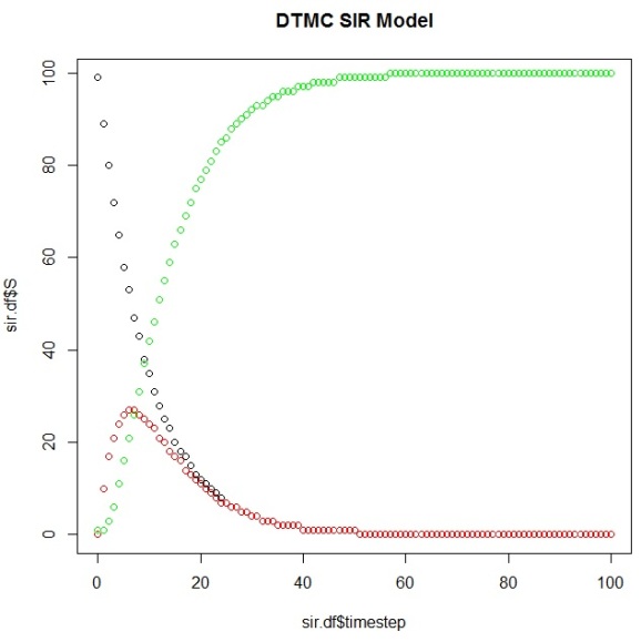
And then plot them to view our simulation results using this DTMC SIR Model:

plot(sir.df$timestep,sir.df$S)
points(sir.df$timestep,sir.df$I, col="red")
points(sir.df$timestep,sir.df$R, col="green")

It’s also possible to use the markovchain package to identify elements of your system as it evolves over time:

&g; absorbingStates(mcSIR)
[1] "R"
> transientStates(mcSIR)
[1] "S" "I"
> steadyStates(mcSIR)
     S I R
[1,] 0 0 1

And you can calculate the first timestep that your Markov Chain reaches its steady state (the “time to absorption”), which your plot should corroborate:

> ab.state  occurs.at  (sir.df[row,]$timestep)+1
[1] 58

You can use this code to change the various transition probabilities to see what the effects are on the outputs yourself (sensitivity analysis). Also, there are methods you can use to perform uncertainty analysis, e.g. putting confidence intervals around your transition probabilities. We won’t do either of these here, nor will we create a Shiny app to run this simulation, despite the significant temptation.