Analyses of Batsmen

The following plots gives the analysis of the 2 Australian and 2 English batsmen. It must be kept in mind that Cooks has more innings than all the rest put together. Smith has the best average, and Warner has the best strike rate

Box Histogram Plot

This plot shows a combined boxplot of the Runs ranges and a histogram of the Runs Frequency

batsmanPerfBoxHist("./smith.csv","S Smith")

batsmanPerfBoxHist("./warner.csv","D Warner")

batsmanPerfBoxHist("./cook.csv","A Cook")

batsmanPerfBoxHist("./root.csv","JE Root")

Plot os 4s, 6s and the type of dismissals

A. Steven Smith

par(mfrow=c(1,3))
par(mar=c(4,4,2,2))
batsman4s("./smith.csv","S Smith")
batsman6s("./smith.csv","S Smith")
batsmanDismissals("./smith.csv","S Smith")

dev.off()
## null device 
##           1

B. David Warner

par(mfrow=c(1,3))
par(mar=c(4,4,2,2))
batsman4s("./warner.csv","D Warner")
batsman6s("./warner.csv","D Warner")
batsmanDismissals("./warner.csv","D Warner")

dev.off()
## null device 
##           1

C. Alistair Cook

par(mfrow=c(1,3))
par(mar=c(4,4,2,2))
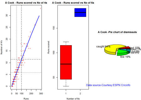
batsman4s("./cook.csv","A Cook")
batsman6s("./cook.csv","A Cook")
batsmanDismissals("./cook.csv","A Cook")

dev.off()
## null device 
##           1

D. J E Root

par(mfrow=c(1,3))
par(mar=c(4,4,2,2))
batsman4s("./root.csv","JE Root")
batsman6s("./root.csv","JE Root")
batsmanDismissals("./root.csv","JE Root")

dev.off()
## null device 
##           1

Relative Mean Strike Rate

In this first plot I plot the Mean Strike Rate of the batsmen. It can be Warner’s has the best strike rate (hit outside the plot!) followed by Smith in the range 20-100. Root has a good strike rate above hundred runs. Cook maintains a good strike rate.

par(mar=c(4,4,2,2))
frames <- list("./smith.csv","./warner.csv","cook.csv","root.csv")
names <- list("Smith","Warner","Cook","Root")
relativeBatsmanSR(frames,names)

Relative Runs Frequency Percentage

The plot below show the percentage contribution in each 10 runs bucket over the entire career.It can be seen that Smith pops up above the rest with remarkable regularity.COok is consistent over the entire range.

frames <- list("./smith.csv","./warner.csv","cook.csv","root.csv")
names <- list("Smith","Warner","Cook","Root")
relativeRunsFreqPerf(frames,names)

Moving Average of runs over career

The moving average for the 4 batsmen indicate the following 1. S Smith is the most promising. There is a marked spike in Performance. Cook maintains a steady pace and is consistent over the years averaging 50 over the years.

par(mfrow=c(2,2))
par(mar=c(4,4,2,2))
batsmanMovingAverage("./smith.csv","S Smith")
batsmanMovingAverage("./warner.csv","D Warner")
batsmanMovingAverage("./cook.csv","A Cook")
batsmanMovingAverage("./root.csv","JE Root")

dev.off()
## null device 
##           1

Runs forecast

The forecast for the batsman is shown below. As before Cooks’s performance is really consistent across the years and the forecast is good for the years ahead. In Cook’s case it can be seen that the forecasted and actual runs are reasonably accurate

par(mfrow=c(2,2))
par(mar=c(4,4,2,2))
batsmanPerfForecast("./smith.csv","S Smith")
batsmanPerfForecast("./warner.csv","D Warner")
batsmanPerfForecast("./cook.csv","A Cook")
## Warning in HoltWinters(ts.train): optimization difficulties: ERROR:
## ABNORMAL_TERMINATION_IN_LNSRCH
batsmanPerfForecast("./root.csv","JE Root")

dev.off()
## null device 
##           1

3D plot of Runs vs Balls Faced and Minutes at Crease

The plot is a scatter plot of Runs vs Balls faced and Minutes at Crease. A prediction plane is fitted

par(mfrow=c(1,2))
par(mar=c(4,4,2,2))
battingPerf3d("./smith.csv","S Smith")
battingPerf3d("./warner.csv","D Warner")

par(mfrow=c(1,2))
par(mar=c(4,4,2,2))
battingPerf3d("./cook.csv","A Cook")
battingPerf3d("./root.csv","JE Root")

dev.off()
## null device 
##           1

Predicting Runs given Balls Faced and Minutes at Crease

A multi-variate regression plane is fitted between Runs and Balls faced +Minutes at crease.

BF <- seq( 10, 400,length=15)
Mins <- seq(30,600,length=15)
newDF <- data.frame(BF,Mins)
smith <- batsmanRunsPredict("./smith.csv","S Smith",newdataframe=newDF)
warner <- batsmanRunsPredict("./warner.csv","D Warner",newdataframe=newDF)
cook <- batsmanRunsPredict("./cook.csv","A Cook",newdataframe=newDF)
root <- batsmanRunsPredict("./root.csv","JE Root",newdataframe=newDF)

The fitted model is then used to predict the runs that the batsmen will score for a given Balls faced and Minutes at crease. It can be seen that Warner sets a searing pace in the predicted runs for a given Balls Faced and Minutes at crease while Smith and Root are neck to neck in the predicted runs

batsmen <-cbind(round(smith$Runs),round(warner$Runs),round(cook$Runs),round(root$Runs))
colnames(batsmen) <- c("Smith","Warner","Cook","Root")
newDF <- data.frame(round(newDF$BF),round(newDF$Mins))
colnames(newDF) <- c("BallsFaced","MinsAtCrease")
predictedRuns <- cbind(newDF,batsmen)
predictedRuns
##    BallsFaced MinsAtCrease Smith Warner Cook Root
## 1          10           30     9     12    6    9
## 2          38           71    25     33   20   25
## 3          66          111    42     53   33   42
## 4          94          152    58     73   47   59
## 5         121          193    75     93   60   75
## 6         149          234    91    114   74   92
## 7         177          274   108    134   88  109
## 8         205          315   124    154  101  125
## 9         233          356   141    174  115  142
## 10        261          396   158    195  128  159
## 11        289          437   174    215  142  175
## 12        316          478   191    235  155  192
## 13        344          519   207    255  169  208
## 14        372          559   224    276  182  225
## 15        400          600   240    296  196  242

batsmanRunsLikelihood("./smith.csv","S Smith")


## Summary of  S Smith 's runs scoring likelihood
## **************************************************
## 
## There is a 40 % likelihood that S Smith  will make  41 Runs in  73 balls over 101  Minutes 
## There is a 36 % likelihood that S Smith  will make  9 Runs in  21 balls over  27  Minutes 
## There is a 24 % likelihood that S Smith  will make  139 Runs in  237 balls over 338  Minutes

batsmanRunsLikelihood("./warner.csv","D Warner")


## Summary of  D Warner 's runs scoring likelihood
## **************************************************
## 
## There is a 11.11 % likelihood that D Warner  will make  134 Runs in  159 balls over 263  Minutes 
## There is a 63.89 % likelihood that D Warner  will make  17 Runs in  25 balls over  37  Minutes 
## There is a 25 % likelihood that D Warner  will make  73 Runs in  105 balls over 156  Minutes

batsmanRunsLikelihood("./cook.csv","A Cook")


## Summary of  A Cook 's runs scoring likelihood
## **************************************************
## 
## There is a 27.72 % likelihood that A Cook  will make  64 Runs in  140 balls over 195  Minutes 
## There is a 59.9 % likelihood that A Cook  will make  15 Runs in  32 balls over  46  Minutes 
## There is a 12.38 % likelihood that A Cook  will make  141 Runs in  300 balls over 420  Minutes

batsmanRunsLikelihood("./root.csv","JE Root")


## Summary of  JE Root 's runs scoring likelihood
## **************************************************
## 
## There is a 28.3 % likelihood that JE Root  will make  81 Runs in  158 balls over 223  Minutes 
## There is a 7.55 % likelihood that JE Root  will make  179 Runs in  290 balls over  425  Minutes 
## There is a 64.15 % likelihood that JE Root  will make  16 Runs in  39 balls over 59  Minutes

Average runs at ground and against opposition

A. Steven Smith

par(mfrow=c(1,2))
par(mar=c(4,4,2,2))
batsmanAvgRunsGround("./smith.csv","S Smith")
batsmanAvgRunsOpposition("./smith.csv","S Smith")

dev.off()
## null device 
##           1

B. David Warner

par(mfrow=c(1,2))
par(mar=c(4,4,2,2))
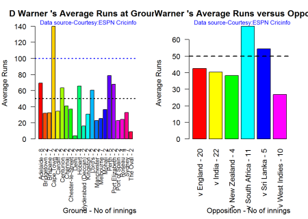
batsmanAvgRunsGround("./warner.csv","D Warner")
batsmanAvgRunsOpposition("./warner.csv","D Warner")

dev.off()
## null device 
##           1

C. Alistair Cook

par(mfrow=c(1,2))
par(mar=c(4,4,2,2))
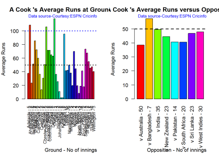
batsmanAvgRunsGround("./cook.csv","A Cook")
batsmanAvgRunsOpposition("./cook.csv","A Cook")

dev.off()
## null device 
##           1

D. J E Root

par(mfrow=c(1,2))
par(mar=c(4,4,2,2))
batsmanAvgRunsGround("./root.csv","JE Root")
batsmanAvgRunsOpposition("./root.csv","JE Root")

dev.off()
## null device 
##           1

Analysis of bowlers

1. Mitchell Johnson (Aus) – Innings-131, Wickets – 299, Econ Rate : 3.28
2. Peter Siddle (Aus) – Innings – 104 , Wickets- 192, Econ Rate : 2.95
3. James Anderson (Eng) – Innings – 199 , Wickets- 406, Econ Rate : 3.05
4. Stuart Broad (Eng) – Innings – 148 , Wickets- 296, Econ Rate : 3.08

Anderson has the highest number of inning and wickets followed closely by Broad and Mitchell who are in a neck to neck race with respect to wickets. Johnson is on the more expensive side though. Siddle has fewer innings but a good economy rate.

Wickets Runs plot

The plot below gives a boxplot of the runs ranges for each of the wickets taken by the bowlers

par(mfrow=c(1,4))
par(mar=c(4,4,2,2))
bowlerWktsRunsPlot("./johnson.csv","Johnson")
bowlerWktsRunsPlot("./siddle.csv","Siddle")
bowlerWktsRunsPlot("./broad.csv","Broad")
bowlerWktsRunsPlot("./anderson.csv","Anderson")

dev.off()
## null device 
##           1

Average wickets in different grounds and opposition

A. Mitchell Johnson

par(mfrow=c(1,2))
par(mar=c(4,4,2,2))
bowlerAvgWktsGround("./johnson.csv","Johnson")
bowlerAvgWktsOpposition("./johnson.csv","Johnson")

dev.off()
## null device 
##           1

B. Peter Siddle

par(mfrow=c(1,2))
par(mar=c(4,4,2,2))
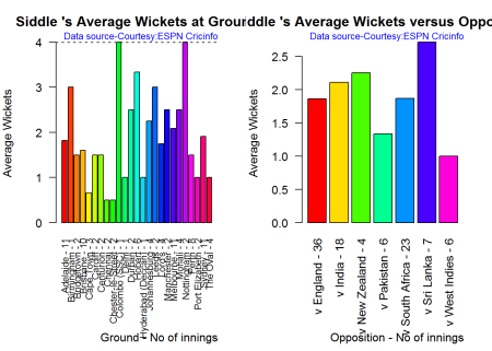
bowlerAvgWktsGround("./siddle.csv","Siddle")
bowlerAvgWktsOpposition("./siddle.csv","Siddle")

dev.off()
## null device 
##           1

C. Stuart Broad

par(mfrow=c(1,2))
par(mar=c(4,4,2,2))
bowlerAvgWktsGround("./broad.csv","Broad")
bowlerAvgWktsOpposition("./broad.csv","Broad")

dev.off()
## null device 
##           1

D. James Anderson

par(mfrow=c(1,2))
par(mar=c(4,4,2,2))
bowlerAvgWktsGround("./anderson.csv","Anderson")
bowlerAvgWktsOpposition("./anderson.csv","Anderson")

dev.off()
## null device 
##           1

Relative bowling performance

The plot below shows that Mitchell Johnson is the mopst effective bowler among the lot with a higher wickets in the 3-6 wicket range. Broad and Anderson seem to perform well in 2 wickets in comparison to Siddle but in 3 wickets Siddle is better than Broad and Anderson.

frames <- list("./johnson.csv","./siddle.csv","broad.csv","anderson.csv")
names <- list("Johnson","Siddle","Broad","Anderson")
relativeBowlingPerf(frames,names)

Relative Economy Rate against wickets taken

Anderson followed by Siddle has the best economy rates. Johnson is fairly expensive in the 4-8 wicket range.

frames <- list("./johnson.csv","./siddle.csv","broad.csv","anderson.csv")
names <- list("Johnson","Siddle","Broad","Anderson")
relativeBowlingER(frames,names)

Moving average of wickets over career

Johnson is on his second peak while Siddle is on the decline with respect to bowling. Broad and Anderson show improving performance over the years.

par(mfrow=c(2,2))
par(mar=c(4,4,2,2))
bowlerMovingAverage("./johnson.csv","Johnson")
bowlerMovingAverage("./siddle.csv","Siddle")
bowlerMovingAverage("./broad.csv","Broad")
bowlerMovingAverage("./anderson.csv","Anderson")

dev.off()
## null device 
##           1

Wickets forecast

par(mfrow=c(2,2))
par(mar=c(4,4,2,2))
bowlerPerfForecast("./johnson.csv","Johnson")
bowlerPerfForecast("./siddle.csv","Siddle")
bowlerPerfForecast("./broad.csv","Broad")
bowlerPerfForecast("./anderson.csv","Anderson")

dev.off()
## null device 
##           1