A simple explanation of rejection sampling in R
[This article was first published on theoretical ecology » Submitted to R-bloggers, and kindly contributed to R-bloggers]. (You can report issue about the content on this page here)
Want to share your content on R-bloggers? click here if you have a blog, or here if you don't.
The central quantity in Bayesian inference, the posterior, can usually not be calculated analytically, but needs to be estimated by numerical integration, which is typically done with a Monte-Carlo algorithm. The three main algorithm classes for doing so are
Want to share your content on R-bloggers? click here if you have a blog, or here if you don't.
- Rejection sampling
- Markov-Chain Monte Carlo (MCMC) sampling
- Sequential Monte Carlo (SMC) sampling
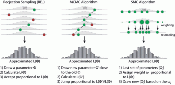
repeat 1. draw random value from the prior 2. calculate likelihood 3. accept value proportional to the likelihoodBecause you accept proportional to your target, the distribution of accepted parameter values will approach the posterior. There is one disadvantage of this method that is obvious – you propose from the whole parameter space, which means that you will typically get a lot of rejections, which is costly (well, it’s called rejection sampling after all). MCMC, in contrast, does a random walk (Markov-chain) in parameter space, and thereby concentrates sampling on the important parameter areas. That is why it is more efficient. But MCMC also has a drawback – because the next step depends on the last step, it’s difficult to parallelize. SMC and rejection sampling, on the other hand, work in parallel anyway and are therefore trivially parallelizable. To see the difference to other sampling methods visually, have a look at this illustration of the three methods, taken from our 2011 EL review
 There are more benefits to rejection sampling than parallelization. For example when using rejection sampling for Approximate Bayesian Computation, there is the subtle but practically relevant advantage that you don’t have to choose the acceptance parameter in advance of the simulations. Finally, rejection sampling is a modern classic. I hope that’s enough motivation.
So, here is how you would do it in R:
An example in R
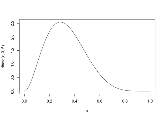
Assume we want to draw from a beta distribution with shape parameters 3,6, which looks like thiscurve(dbeta(x, 3,6),0,1)
 To do this, we first create a data.frame with 100000 random values between 0 and 1, and calculate their beta density values
sampled <- data.frame(proposal = runif(100000,0,1))
sampled$targetDensity <- dbeta(sampled$proposal, 3,6)
Now, accept proportional to the targetDensity. It’s easiest if we calculate the highest density value, and then accept the others in relation to that
maxDens = max(sampled$targetDensity, na.rm = T)
sampled$accepted = ifelse(runif(100000,0,1) < sampled$targetDensity / maxDens, TRUE, FALSE)
Plot the result
hist(sampled$proposal[sampled$accepted], freq = F, col = "grey", breaks = 100)
curve(dbeta(x, 3,6),0,1, add =T, col = "red")
 A copy of the entire code is available on GitHub here
To leave a comment for the author, please follow the link and comment on their blog: theoretical ecology » Submitted to R-bloggers.
R-bloggers.com offers daily e-mail updates about R news and tutorials about learning R and many other topics. Click here if you're looking to post or find an R/data-science job.
Want to share your content on R-bloggers? click here if you have a blog, or here if you don't.
