The previous article introduced the sensitivity and elasticity to seasonal matrix model of imaginary annual plant.  Both sensitivity and elasticity are partial derivatives.  This means the values can only predict a change of λ with respect to a small change of a element.

To know how λ will affected by a large shift or changes of multiple elements, the simplest way is to calculate each λ for each case.

R can easily do this.

The λ can also be solved analytically, because this example is very simple.  Let’s check whether both results match.

We have four elements:

seed  <- 0.9^4  # Seed surviving rate; annual
germ  <- 0.3    # Germination rate; spring
plant <- 0.05   # Plant surviving rate; from germination to mature
yield <- 100    # Seed production number; per matured plant

The function lambda and A.spring were defined in the previous article:

lambda <- function(A) eigen(A)$values[1]
# and so on. 

Let’s change one of them; the seed:

n <- 100
lambdas <- numeric(n)
seeds <- seq(from=0, to=1, length.out=n)^2
for(i in 1:n) { 
  seed <- seeds[i] 
  lambdas[i] <- lambda(A.spring()) 
}
seed  <- 0.9^4  # restore the initial value

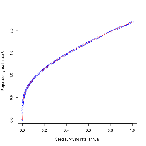
plot(seeds, lambdas, ylab='Population growth rate λ', 
     xlab='Seed surviving rate; annual', col='blue')
abline(a=1, b=0)

Blue plots indicate the result of simulation.

From analytic solution:

# λ = 0.7 * seed + 1.5 * seed^(1/4)

Drawing this curve with red line on the blue plots.

curve(0.7 * x + 1.5 * x^(1/4), add=T, 
      from=min(seeds), to=max(seeds), col='red')

Both results met very well.

The germ:

germs <- seq(from=0, to=1, length.out=n)
for(i in 1:n) { 
  germ <- germs[i]
  lambdas[i] <- lambda(A.spring()) 
}
germ  <- 0.3    # restore the initial value

plot(germs, lambdas, ylab='Population growth rate λ', 
     xlab='Germination rate; spring', col='blue')
abline(a=1, b=0)

From analytic solution:

# λ = 0.6561 + 3.8439 * germ
curve(0.6561 + 3.8439 * x, add=T, 
      from=min(germs), to=max(germs), col='red')

Both results met very well.

The plant:

plants <- seq(from=0, to=0.1, length.out=n)
for(i in 1:n) { 
  plant <- plants[i]
  lambdas[i] <- lambda(A.spring()) 
}
plant <- 0.05   # restore the initial value

plot(plants, lambdas, ylab='Population growth rate λ', 
     xlab='Plant surviving rate; from germination to mature', 
     col='blue')
abline(a=1, b=0)

From analytic solution:

# λ = 0.45927 + 27 * plant
curve(0.45927 + 27 * x, add=T, 
      from=min(plants), to=max(plants), col='red')

Both results met very well.

The yield:

yields <- seq(from=0, to=200, length.out=n)
for(i in 1:n) { 
  yield <- yields[i]
  lambdas[i] <- lambda(A.spring()) 
}
yield <- 100    # restore the initial value

plot(yields, lambdas, ylab='Population growth rate λ', 
     xlab='Seed production number; per matured plant', 
     col='blue')
abline(a=1, b=0)

From analytic solution:

# λ = 0.45927 + 0.0135 * yield
curve(0.45927 + 0.0135 * x, add=T, 
      from=min(yields), to=max(yields), col='red')

Both results met very well.

The seed and the germ:

n <- 64
lambdas <- matrix(nrow=n, ncol=n)

plant <- 0.05   # Plant surviving rate; from germination to mature
yield <- 100    # Seed production number; per matured plant

seeds <- seq(from=0, to=1, length.out=n)^2
germs <- seq(from=0, to=1, length.out=n)^2

for(ro in 1:n) for(co in 1:n) { 
  seed <- seeds[ro]
  germ <- germs[co]
  lambdas[ro, co] <- lambda(A.spring()) 
}
contour(x=seeds, y=germs, z=lambdas, main='λ', 
        xlab='Seed surviving rate; annual', 
        ylab='Germination rate; spring')

The seed and the plant:

n <- 64
lambdas <- matrix(nrow=n, ncol=n)

germ  <- 0.3    # Germination rate; spring
yield <- 100    # Seed production number; per matured plant

seeds <- seq(from=0, to=1, length.out=n)^2
plants <- seq(from=0, to=0.3, length.out=n)^2

for(ro in 1:n) for(co in 1:n) { 
  seed <- seeds[ro]
  plant <- plants[co]
  lambdas[ro, co] <- lambda(A.spring()) 
}
contour(x=seeds, y=plants, z=lambdas, 
        xlab='Seed surviving rate; annual', main='λ', 
        ylab='Plant surviving rate; from germination to mature')

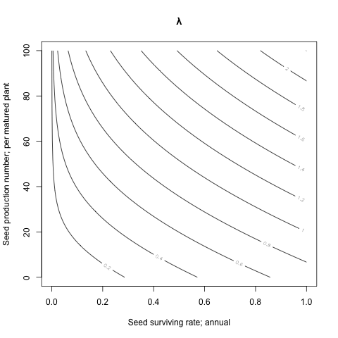
The seed and the yield:

n <- 64
lambdas <- matrix(nrow=n, ncol=n)

germ  <- 0.3    # Germination rate; spring
plant <- 0.05   # Plant surviving rate; from germination to mature

seeds <- seq(from=0, to=1, length.out=n)^2
yields <- seq(from=0, to=sqrt(100), length.out=n)^2

for(ro in 1:n) for(co in 1:n) { 
  seed <- seeds[ro]
  yield <- yields[co]
  lambdas[ro, co] <- lambda(A.spring()) 
}
contour(x=seeds, y=yields, z=lambdas, main='λ', 
        xlab='Seed surviving rate; annual', 
        ylab='Seed production number; per matured plant')