In the past week, colleagues of mine and me started using the lme4-package to compute multi level models. This inspired me doing two new functions for visualizing random effects (as retrieved by ranef()) and fixed effects (as retrieved by fixed()) of (generalized) linear mixed effect models.

The upcoming version of my sjPlot package will contain two new functions to plot fitted lmer and glmer models from the lme4 package: sjp.lmer and sjp.glmer (not that surprising function names). Since I’m new to mixed effects models, I would appreciate any suggestions on how to improve the functions, which results are important to report (plot) and so on. Furthermore, I’m not sure whether my approach of computing confident intervals for random effects is the best? I have used following code to computer confident intervals for the estimates returned by the lme4::ranef() function (bases on this stackoverflow answer):

coev <- as.matrix(lme4::vcov.merMod(fit))
tmp <- as.data.frame(cbind(OR = exp(mydf.ef[,i]),
                     lower.CI = exp(mydf.ef[,i] - (1.96 * sqrt(diag(coev))[i])),
                     upper.CI = exp(mydf.ef[,i] + (1.96 * sqrt(diag(coev))[i]))))

The update to version 1.6 of sjPlot is still in development (feature-freeze, mostly fixes now), however, you can download the latest snapshot from GitHub (see also this post for further information).

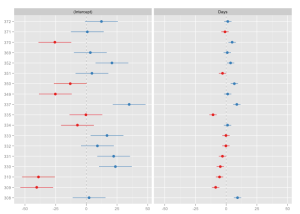
Now to some examples. First, an example model is fitted and the random effects (default) for each predictor are plotted as “forest plot”:

# fit model
library(lme4)
fit <- lmer(Reaction ~ Days + (Days | Subject), sleepstudy)
# simple plot
sjp.lmer(fit)

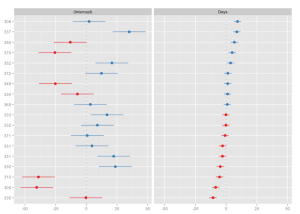
Sorting a predictor (i.e. estimates of a facet) is done by specifying the predicor’s name as sort parameter.

sjp.lmer(fit, sort = "Days")

Each facet plot can also be plotted as single plot, when facet.grid is set to FALSE. In this case, it is possible to sort the estimates for each plots. See following example from the sjp.glmer function:

library(lme4)
# create binary response
sleepstudy$Reaction.dicho <- sju.dicho(sleepstudy$Reaction, 
                                       dichBy = "md")
# fit model
fit <- glmer(Reaction.dicho ~ Days + (Days | Subject),
             sleepstudy,
             family = binomial("logit"))
sjp.setTheme(theme = "forest")
sjp.glmer(fit, 
          facet.grid = FALSE, 
          sort = "sort.all")

Plotting the fixed effects is not much spectacular.

sjp.glmer(fit, 
          type = "fe", 
          sort = TRUE)

Random and fixed effects are plotted in the way shown above. Are there any other or better plot options for visualizing mixed effects models? Any suggestions are welcome…