Stage abundances, eigenvector of population matrix
Want to share your content on R-bloggers? click here if you have a blog, or here if you don't.
The previous article introduced the seasonal matrices and the population growth rate λ of imaginary annual plant. This article focuses on the meaning of the eigenvector at first, and then focuses on the reduction of seasons from 4 to 2.
4. Population structure
The eigenvector corresponding to the dominant eigenvalue λ gives the stable population structure.
population.structure <- function(A) eigen(A)$vectors[,1]

> population.structure(A.spring())
[1] 0.3939193 0.9191450
> population.structure(A.summer())
[1] 0.04756515 0.99886814
> population.structure(A.autumn())
[1] 0.02644577 0.99965025
> population.structure(A.winter())
[1] 1
So, at spring, seedling number vs. dormant seed number is 0.394:0.919 = 30%:70%. This ratio is exactly equal to the spring germination rate.
At summer, flowering plant number vs. dormant seed number is 0.0476:0.999 = 4.5%:95.5%. So, when we watch flowers of this imaginary plant in summer, 21-fold seeds are sleeping in soil.
At autumn, seed production plant number vs. dormant seed number is 0.0264:0.9997 = 2.6%:97.4%. Mature plants are only 2.6% of total population. Because seed production number of this imaginary plant is 100 seeds per plant, this small ratio of reproductive stage adults is enough to increase the population.
At winter, because the population has only one stage, the eigenvector is a scalar 1. The 100% of the population is dormant seed.
5. Reduction to two seasonal matrices model
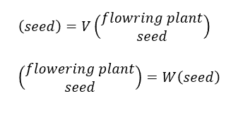
The previous four seasonal model can be simplified to two seasonal model, because there are no important stage transitions from spring to autumn. The transition matrices P and Q are both diagonal; only surviving rate of plant and dormant seed are described respectively. So spring, summer and autumn can be summarized to a single period, such as, ‘summer’.
| Season | Stages |
|---|---|
| Summer | flowering plants, seeds |
| Winter | seeds |
The matrix V and W are same as products RQ and PS respectively.
> V <- R %*% Q
[,1] [,2]
[1,]   50 0.81
> W <- P %*% S
[,1]
[1,] 0.027
[2,] 0.567
The results are same as the four seasonal ones shown previously.
> eigen(W %*% V)
$values
[1] 1.80927 0.00000

$vectors
[,1]        [,2]
[1,] 0.04756515 -0.01619787
[2,] 0.99886814  0.99986881

> eigen(V %*% W)
$values
[1] 1.80927

$vectors
[,1]
[1,]    1
R-bloggers.com offers daily e-mail updates about R news and tutorials about learning R and many other topics. Click here if you're looking to post or find an R/data-science job.
Want to share your content on R-bloggers? click here if you have a blog, or here if you don't.


