Space, a wise man once said, is the final frontier.

Not the Buzz Alrdin/Light Year, Neil deGrasse Tyson kind (but seriously, have you seen Cosmos?). Geographic space. Distances have been finding their way into metrics since the cavemen (probably). GIS seem to make nearly every science way more fun…and accurate!

Most of my research deals with spatial elements of real estate modeling. Unfortunately, “location, location, location” has become a clichéd way to begin any paper or presentation pertaining to spatial real estate methods. For you geographers, it’s like setting the table with Tobler’s first law of geography: a quick fix (I’m not above that), but you’ll get some eye-rolls. But location is important!

One common method of taking location and space into account in real estate valuation models is by including distance coefficients (e.g. distance to downtown, distance to center of city). The geographers have this straight-line calculation of distance covered,  and R can spit out distances between points in a host of measurement systems (euclidean, great circle, etc.). This straight-line distance coefficient is a helpful tool when you want to help reduce some spatial autocorrelation in a model, but it doesn’t always tell the whole story by itself (please note: the purpose of this post is to focus on the tools of R and introduce elements of spatial consideration into modeling. I’m purposefully avoiding any lengthy discussions on spatial econometrics or other spatial modeling techniques, but if you would like to learn more about the sheer awesomeness that is spatial modeling, as well as the pit-falls/pros and cons of each, check out Luc Anselin and Stewart Fotheringham for starters. I also have papers being publishing this fall and would be more than happy to forward you a copy if you email me. They are:

Bidanset, P. & Lombard, J. (2014). The effect of kernel and bandwidth specification in geographically weighted regression models on the accuracy and uniformity of mass real estate appraisal. Journal of Property Tax Assessment & Administration. 11(3). (copy on file with editor).

and

Bidanset, P. & Lombard, J. (2014). Evaluating spatial model accuracy in mass real estate appraisal: A comparison of geographically weighted regression (GWR) and the spatial lag model (SLM). Cityscape: A Journal of Policy Development and Research. 16(3). (copy on file with editor).).

Straight-line distance coefficients certainly can help account for location, as well as certain distance-based effects on price. Say you are trying to model negative externalities of a landfill in August, assuming wind is either random or non-existent, straight-line distance from the landfill to house sales could help capture the cost of said stank. Likewise with capturing potential spill-over effects of an airport  – the sound of jets will diminish as space increases, and the path of sound will be more or less a straight line.

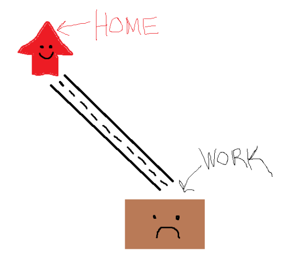
But  again, certain distance-based elements cannot be accurately represented with this method. You may expect ‘distance to downtown’ to have an inverse relationship with price: the further you out you go, more of a cost is incurred (in time, gas, and overall inconvenience) getting to work and social activities, so demand for these further out homes decreases, resulting in cheaper priced homes (pardon the hasty economics). Using straight-line distances to account commute in a model, presents some problems (aside: There is nary a form of visualization capable of presenting one’s point more professionally than Paint, and as anyone who has ever had the misfortune of being included in a group email chain with me knows, I am a bit of a Paint artist.). If a trip between a person’s work and a person’s home followed a straight line, this would be less of a problem (artwork below).

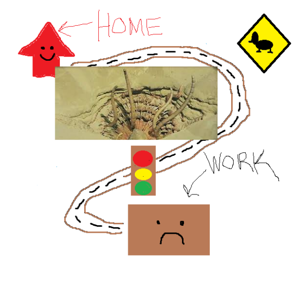
But we all know commuting is more complicated than this. There could be a host of things between you and your place of employment that would make a straight-line distance coefficient an inept method of quantifying this effect on home values … such as a lake:

… or a Sarlacc pit monster:

Some cutting edge real estate valuation modelers are now including a ‘drive time’ variable. DRIVE TIME! How novel is that? This presents a much more accurate way to account for a home’s distance – as a purchaser would see it – from work, shopping, mini-golf, etc. Sure it’s been available in (expensive) ESRI packages for some time, but where is the soul in that? The altruistic R community has yet again risen to the task.

To put some real-life spin on the example above, let’s run through a very basic regression model for modeling house prices.

sample = read.csv("C:/houses.csv", header=TRUE)
model1 <- lm(ln.ImpSalePrice. ~ TLA + TLA.2 + Age + Age.2 + quality + condition, data = sample)

We read in a csv file “houses” that is stored on the C:/ drive and name it “sample”. You can name it anything, even willywonkaschocolatefactory. We’ll name the first model “model1″. The dependent variable, ln.ImpSalePrice.,  is a log form of the sale price. TLA is ‘total living area’ in square feet. Age is, well, age of the house, and quality and condition are dummy variables. The squared variables of TLA and Age are to capture any diminishing marginal returns.

AIC stands for ‘Akaike information criterion’. Some guy from Japan coined it in the 70’s and it’s a goodness-of-fit measurement to compare models used on the same sample (the lower the AIC, the better).

> AIC(model1)
[1] 36.35485

The AIC of model1 is 36.35.

Now we are going to create some distance variables to add to the model. First we’ll do the straight-line distances. We make a matrix  called “origin” consisting of  start-points, which in this case is the lat/long of each house in our dataset.

origin <- matrix(c(sample$lat, sample$lon), ncol=2)

We next create a destination – to where we will be measuring the distance. For this example, I decided to measure the distance to a popular shopping mall downtown (why not?). I obtained the lat/long coordinates for the mall by right clicking on it in Google Maps and clicking “whats here?” (also could’ve geocoded in R).

destination <- c(36.84895, -76.288018)

Now we use the  spDistsN1 function to calculate the distance. We denote longlat=TRUE so we can get the value from origin to destination in kilometers. The second line just adds this newly created column of distances to our dataset and names it dist.

km <- spDistsN1(origin, destination, longlat=TRUE)
sample$dist <- km

This command I learned from a script on Github – initially committed by Peter Schmiedeskamp – which alerted me to the fact that R was capable of grabbing drive-times from the Google Maps API.  You can learn a great deal from his/their work so give ‘em a follow!

library(ggmap)
library(plyr)

google_results <- rbind.fill(apply(subset(sample, select=c("location", "locMall")), 1, function(x) mapdist(x[1], x[2], mode="driving")))

location is the column containing each house’s lat/long coordinates, in the following format (36.841287,-76.218922). locMall is a column in my data set with the lat/long coords of the mall in each row. Just to clarify: each cell in this column had the exact same value, while each cell of “location” was different.  Also something amazing: mode can either be “driving,” “walking,” or “bicycling”!

Now let’s look at the results:

> head(google_results,4)
           from                        to          m     km    miles seconds minutes
1 (36.901373,-76.219024) (36.848950, -76.288018) 10954 10.954 6.806816 986 16.433333
2 (36.868871,-76.243859) (36.848950, -76.288018) 7279 7.279 4.523171 662 11.033333
3 (36.859805,-76.296122) (36.848950, -76.288018) 2101 2.101 1.305561 301 5.016667
4 (36.938692,-76.264474) (36.848950, -76.288018) 12844 12.844 7.981262 934 15.566667
    hours
1 0.27388889
2 0.18388889
3 0.08361111
4 0.25944444

Amazing, right? And we can add this to our sample and rename it “newsample”:

newsample <- c(sample, google_results)

Now let’s add these variables to the model and see what happens.

model2 <- lm(ln.ImpSalePrice. ~ TLA + TLA.2 + Age + Age.2 + quality+ condition + dist,data = newsample)


> AIC(model2)
[1] 36.44782

Gah, well, no significant change. Hmm…let’s try the drive-time variable…

model3 <- lm(ln.ImpSalePrice. ~ TLA + TLA.2 + Age + Age.2 + quality + condition + minutes,data = newsample)


> AIC(model3)
[1] 36.10303

Hmm…still no dice. Let’s try them together.

> AIC(model3)
model4 <- lm(ln.ImpSalePrice. ~ TLA + TLA.2 + Age + Age.2 + quality + condition + minutes + dist,data = newsample)


> AIC(model4)
[1] 32.97605

Alright! AIC has been reduced by more than 2 so they together have a statistically significant effect on the model.

Of course this is a grossly reduced model, and would never be used for actual valuation/appraisal purposes, but it does lay elementary ground work for creating distance-based variables, integrating them, and demonstrating their ability to marginally improve models.

Thanks for reading. So to bring back Cap’n Kirk, I think a frontier more ultimate than space, in the modeling sense,  is space-time – not Einstein’s, rather ‘spatiotemporal’.  That will will be for another post!

Toodles,

Paul