At the CLRS last year, Glenn Meyers talked about something very near to my heart: a skewed normal distribution. In loss reserving (and I'm sure, many other contexts) standard linear regression is less than ideal as it presumes that deviations from the mean are equally distributed. We rarely expect this assumption to hold (though we should always test it!). Application of a log transform is one way to address this, but that option isn't available for negative observations. Negative incremental reported losses are very common and even negative payments which arise from salvage, subrogation or other factors happen often enough that (in my view) the log transform isn't an attractive option.

Meyers gave a talk where he described (among other things) the lognormal-normal mixture. That presentation, Stochastic Loss Reserving with Bayesian MCMC Models, is worth any actuary's time. The idea is simplicity itself. Z is lognormally distributed, with parameters mu and theta. X is normally distributed with parameters Z and delta.

Let's have a look at this distribution. Well, actually that's easier said than done. Here are the equations:

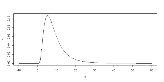
So Z is easy, it's just a lognormal. In fact, here it is:

sigma = 0.6
mu = 2
x = seq(-10, 60, length.out = 500)
Z = dlnorm(x, mu, sigma)
plot(x, Z, type = "l")

X for the expected value of Z is also easy. Here it is:

expZ = exp(mu + sigma^2/2)
delta = 3
pdfX = dnorm(x, expZ, delta)
plot(x, pdfX, type = "l")

Here, we've produced a normal centered around the expected value of the original lognormal distribution. Not skewed and not all that interesting. What we want is a distribution wherein the mean of the normal is itself a random variable. To get that, we have three options: one lazy, one easy and one. I'll show the lazy one first.

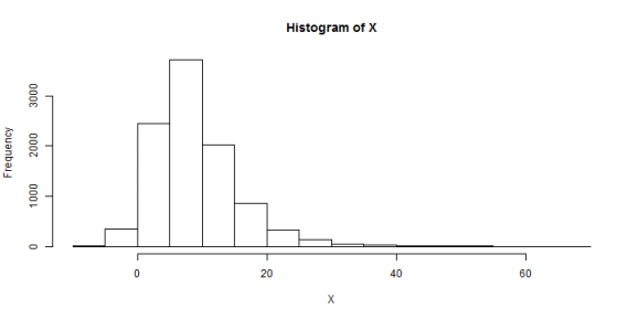
The lazy one is to randomly sample from Z and then feed that to X. We end up with a histogram which approximates a density function.

samples = 10000
Z = rlnorm(samples, mu, sigma)
X = rnorm(samples, Z, delta)
hist(X)

That's undoubtedly skew and might even correspond to Glenn's graph on slide 36. But that was lazy. The easy way is to repeat a procedure similar to what I did a week ago when demonstrating a Bayesian model which combined a lognormal and an exponential. Here, we just calculate the joint density over a subspace of the probability domain, normalize it and then compute the marginal.

plotLength = 250
Z = seq(0.001, 40, length.out = plotLength)
X = seq(-10, 40, length.out = plotLength)

dfJoint = expand.grid(Z = Z, X = X)

dfJoint$Zprob = dlnorm(dfJoint$Z, mu, sigma)
dfJoint$Xprob = dnorm(dfJoint$X, dfJoint$Z, delta)
dfJoint$JointProb = with(dfJoint, Zprob * Xprob)
dfJoint$JointProb = dfJoint$JointProb/sum(dfJoint$JointProb)

jointProb = matrix(dfJoint$JointProb, plotLength, plotLength, byrow = TRUE)

filled.contour(x = X, y = Z, z = jointProb, color.palette = heat.colors, xlab = "X", 
    ylab = "Z")

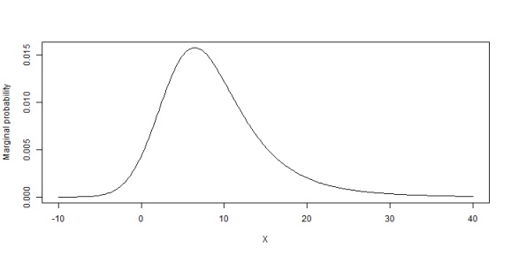
Groovy. X can be anything, but higher values of Z will pull it to the right. Here's the marginal distribution of X.

library(plyr)
marginalX = ddply(dfJoint[, c("X", "JointProb")], .variables = "X", summarize, 
    marginalProb = sum(JointProb))
plot(marginalX$X, marginalX$marginalProb, type = "l", xlab = "X", ylab = "Marginal probability")

The hard way is to sit down with pen and paper and work this out algebraically. I tried. I worked through a few ugly integrations did some research on the interweb and have concluded that if there is a closed form solution, it's not something that people spend a great deal of time talking about. I will point to this paper and this website as material that I'd like to get better acquainted with. It would appear that this comes up in financial and time series analysis. No surprises there, I think there are similar reasons to need this sort of distribution.

For the record, here's what that integrand looks like.

If you know how to integrate that over Z, please let me know.

If you've made it this far, odds are good that you're an actuary, a stats nerd or both. Whatever you are, take a moment to thank heaven for Glenn Meyers, who's both. He's made tremendous contributions to actuarial literature and we're all the better for it.

Session info:

## R version 3.0.2 (2013-09-25)
## Platform: x86_64-w64-mingw32/x64 (64-bit)
## 
## locale:
## [1] LC_COLLATE=English_United States.1252 
## [2] LC_CTYPE=English_United States.1252   
## [3] LC_MONETARY=English_United States.1252
## [4] LC_NUMERIC=C                          
## [5] LC_TIME=English_United States.1252    
## 
## attached base packages:
## [1] stats     graphics  grDevices utils     datasets  methods   base     
## 
## other attached packages:
## [1] knitr_1.5        RWordPress_0.2-3 plyr_1.8        
## 
## loaded via a namespace (and not attached):
## [1] evaluate_0.5.1 formatR_0.10   RCurl_1.95-4.1 stringr_0.6.2 
## [5] tools_3.0.2    XML_3.98-1.1   XMLRPC_0.3-0