Need a Hanukkah or Christmas gift for an R analyst? You could do loads worse than Applied Spatial Data Analysis with R by Bivand, Pebesma and Gomez-Rubio. I don't have my copy yet- I'm still working through all of the other books I've bought this year- but I'll likely pick it up sometime early in 2014. Why? Because I love maps. I also love the sp package that they created. I don't have a strong working knowledge of it yet, but I have found a paper by Zack Almquist to be very useful in working through the basics. Here's a quick example using US census data. Note that if you want to download the Almquist packages that they are huge.

library(UScensus2010)
library(UScensus2010county)

What I'd like to do is see where the oldest Americans live. This package will give us 51 shapefiles, so doing this by state is straightforward. For openers, let's have a look at Florida. To spare myself typing the crazy field names, I'll code a couple helper functions.

data(florida.county10)

Over65 = function(dfCensus) {
    Over65 = dfCensus$H0170009 + dfCensus$H0170010 + dfCensus$H0170011
    Over65 = Over65 + dfCensus$H0170019 + dfCensus$H0170020 + dfCensus$H0170021
    Over65
}

PercentOver65 = function(dfCensus) {
    PercentOver65 = Over65(dfCensus)/dfCensus$H0170001
}
florida.county10$Over65 = Over65(florida.county10)
florida.county10$PercentOver65 = PercentOver65(florida.county10)
florida.county10$PercentOver65 = PercentOver65(florida.county10)

The USCensus choropleth() function works well for me most of the time, but I get an error on the breaks that I use often enough that I've coded my own. This is probably something that I'm doing wrong, but it's a nice exercise to get the choropleths to look right. Actually, I'm fairly sure that I figured out how to set the colors from some code that I read on is.R()'s advent calendaR from last year.

library(RColorBrewer)
library(classInt)

MyChoropleth = function(sp, dem, palette, ...) {
    df = sp@data
    brks = classIntervals(df[, dem], n = length(palette), style = "quantile")
    brks = brks$brks

    sp$MyColor = palette[findInterval(df[, dem], brks, all.inside = TRUE)]
    plot(sp, col = sp$MyColor, axes = F, ...)
}

myPalette = brewer.pal(9, "Blues")
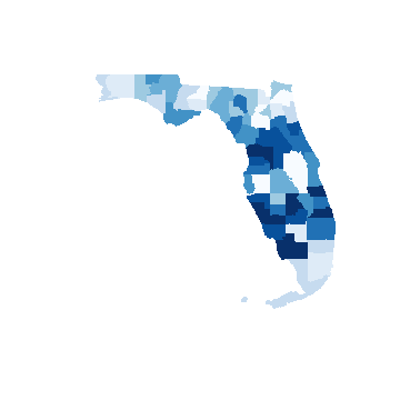
MyChoropleth(florida.county10, "PercentOver65", myPalette, border = "transparent")

So there are fewer seniors in the southernmost part of the state. Given the urban character of a city like Miami, that seems consistent. But how does Florida compare to the rest of the US? This will take a bit more work. First, we'll need to load all of the states data and calculate the over 65 percent. We'll then need to merge all of the states into one very large spatial polygons data frame.

data(states.names)
lower48 = states.names[!states.names %in% c("alaska", "hawaii", "district_of_columbia")]
lower48 = paste0(lower48, ".county10")

data(list = lower48[1])
spLower48 = get(lower48[1])
rm(list = lower48[1])
for (i in 2:48) {
    data(list = lower48[i])
    spLower48 = spRbind(spLower48, get(lower48[i]))
    rm(list = lower48[i])
}
spLower48$PercentOver65 = PercentOver65(spLower48)
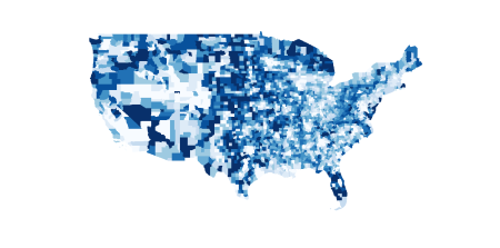
MyChoropleth(spLower48, "PercentOver65", myPalette, border = "transparent")

This code works when I run it in RStudio, but I'm not able to get it to run with knitr. Suggestions welcome. In the meantime, I've had to upload the image to WordPress the old fashioned way.

The resolution is fairly dreadful. Given the lateness of the hour and the length of time it takes R to process all that data and imagery, I'm going to leave well enough alone. Suggestions for improvement are welcome. What's there suggests that Florida has a well-earned reputation for being a favorite place to live for seniours, but there are plenty of older folks in the midwest, as well as Arizona and Nevada. If I had my way, I'd retire somewhere in Europe. It's probably the only way I'll collect anything from my German pension.

Tomorrow I'll begin a lengthy look at the career of actor Michael Caine.

citation("UScensus2010county")

## 
## To cite UScensus2000 in publications use:
## 
##   Zack W. Almquist (2010). US Census Spatial and Demographic Data
##   in R: The UScensus2000 Suite of Packages. Journal of Statistical
##   Software, 37(6), 1-31. URL http://www.jstatsoft.org/v37/i06/.
## 
## A BibTeX entry for LaTeX users is
## 
##   @Article{,
##     title = {US Census Spatial and Demographic Data in {R}: The {UScensus2000} Suite of Packages},
##     author = {Zack W. Almquist},
##     journal = {Journal of Statistical Software},
##     year = {2010},
##     volume = {37},
##     number = {6},
##     pages = {1--31},
##     url = {http://www.jstatsoft.org/v37/i06/},
##   }

sessionInfo()

## R version 3.0.2 (2013-09-25)
## Platform: x86_64-w64-mingw32/x64 (64-bit)
## 
## locale:
## [1] LC_COLLATE=English_United States.1252 
## [2] LC_CTYPE=English_United States.1252   
## [3] LC_MONETARY=English_United States.1252
## [4] LC_NUMERIC=C                          
## [5] LC_TIME=English_United States.1252    
## 
## attached base packages:
## [1] stats     graphics  grDevices utils     datasets  methods   base     
## 
## other attached packages:
## [1] knitr_1.4.1             RWordPress_0.2-3        classInt_0.1-21        
## [4] RColorBrewer_1.0-5      UScensus2010county_1.00 UScensus2010_0.11      
## [7] foreign_0.8-55          maptools_0.8-27         sp_1.0-13              
## 
## loaded via a namespace (and not attached):
##  [1] class_7.3-9     digest_0.6.3    e1071_1.6-1     evaluate_0.4.7 
##  [5] formatR_0.9     grid_3.0.2      lattice_0.20-23 RCurl_1.95-4.1 
##  [9] stringr_0.6.2   tools_3.0.2     XML_3.98-1.1    XMLRPC_0.3-0