On vacation with my family this week and that means I have a few minutes now and again to read. One of the books I brought along is Christopher Gandrud’s excellent “Reproducible Research with R and RStudio”.

Looking for some data as a test project, I latched onto Hurricane data. Folly Beach was hit pretty hard by hurricane Hugo in 1989. It’s easy (though not terribly enjoyable) to imagine the damage such an event would do to a small coastal community like this. What’s the likelihood that a hurricane will hit here again? What does it depend on? Obviously smarter minds than mine are hard at work on this. I can’t hope to eclipse their knowledge, but this is a bit of fun to think about.

The project is available on GitHub here: https://github.com/PirateGrunt/Hurricane. If Gandrud has taught me anything, everything that I do will be easy to reproduce. As a first step, I show that (for this data) decade is a useful predictor for the number of hurricanes per year. I’m going to be a bit lazy and paste the HTML for the basic analysis file into this blog post. The raw code is available on GitHub.

First, read in the data for number of hurricanes by year and then fit a poisson.

setwd("~/GitHub/Hurricane/Data")

df = read.csv("HurricaneByYear.csv")

fitPoissonAll = glm(Num ~ 1, family = poisson, data = df)
summary(fitPoissonAll)

## 
## Call:
## glm(formula = Num ~ 1, family = poisson, data = df)
## 
## Deviance Residuals: 
##    Min      1Q  Median      3Q     Max  
## -3.789  -1.521  -0.485   0.733   5.098  
## 
## Coefficients:
##             Estimate Std. Error z value Pr(>|z|)    
## (Intercept)   2.3546     0.0243      97   <2e-16 ***
## ---
## Signif. codes:  0 '***' 0.001 '**' 0.01 '*' 0.05 '.' 0.1 ' ' 1
## 
## (Dispersion parameter for poisson family taken to be 1)
## 
##     Null deviance: 434.14  on 160  degrees of freedom
## Residual deviance: 434.14  on 160  degrees of freedom
## AIC: 1093
## 
## Number of Fisher Scoring iterations: 4


lambda = exp(fitPoissonAll$coefficients[1])

We’ll note that the estimated lambda is equal to the sample mean.

mean(df$Num)

## [1] 10.53

lambda

## (Intercept) 
##       10.53

Now, we’ll plot the number of hurricanes by year along with a line for the poisson parameter

plot(df$Year, df$Num, pch = 19)
abline(lambda, 0)  

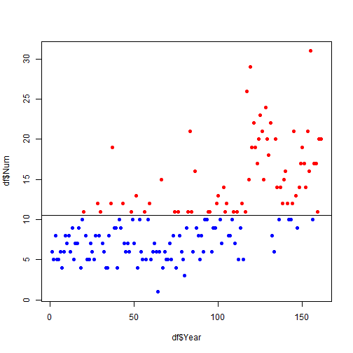
Hmm, looks like the more recent years have more points above the fit line. Let’s have a look. We’ll color the points so that observations above the mean are red and observations below the mean are blue.

ltAvg = ifelse(df$Num < lambda, "blue", "red")
summary(ltAvg)

##    Length     Class      Mode 
##       161 character character

table(ltAvg)

## ltAvg
## blue  red 
##   95   66

plot(df$Year, df$Num, pch = 19, col = ltAvg)
abline(lambda, 0)  

Yep, there definitely appear to be more hurricanes in recent years. Let’s add a parameter for the decade to see if it improves the fit.

df$Decade = trunc(df$Year/10)
df$Decade = df$Decade - min(df$Decade)

summary(df$Decade)

##    Min. 1st Qu.  Median    Mean 3rd Qu.    Max. 
##    0.00    4.00    8.00    7.65   12.00   16.00

fitPoissonByDecade = glm(Num ~ 1 + Decade, family = poisson, data = df)
summary(fitPoissonByDecade)
## 
## Call:
## glm(formula = Num ~ 1 + Decade, family = poisson, data = df)
## 
## Deviance Residuals: 
##    Min      1Q  Median      3Q     Max  
## -3.382  -0.947  -0.180   0.639   3.932  
## 
## Coefficients:
##             Estimate Std. Error z value Pr(>|z|)    
## (Intercept)  1.76656    0.05484    32.2   <2e-16 ***
## Decade       0.06999    0.00538    13.0   <2e-16 ***
## ---
## Signif. codes:  0 '***' 0.001 '**' 0.01 '*' 0.05 '.' 0.1 ' ' 1
## 
## (Dispersion parameter for poisson family taken to be 1)
## 
##     Null deviance: 434.14  on 160  degrees of freedom
## Residual deviance: 259.70  on 159  degrees of freedom
## AIC: 920.7
## 
## Number of Fisher Scoring iterations: 4

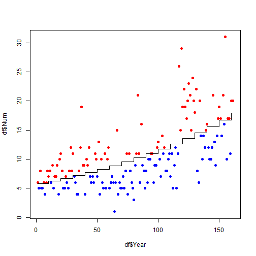
The null deviance decreases far more than would be expected if the decade had no predictive power. We’ll plot the prediction against the observations. A step function will make the most sense visually.

df$DecadePredict = exp(predict(fitPoissonByDecade))

plot(df$Year, df$Num, pch = 19)
lines(df$Year, df$DecadePredict, type = "s")

ltAvg = ifelse(df$Num < df$DecadePredict, "blue", "red")
plot(df$Year, df$Num, pch = 19, col = ltAvg)
lines(df$Year, df$DecadePredict, type = "s") 

So, there appear to be more hurricanes in recent decades. Is this because of some meterological or atmospheric change? Or does it have something to do with the way observations have been collected? I’ll look into that next.