Latent Gaussian Models and INLA

Posted on October 16, 2013 by thiagogm in R bloggers | 0 Comments

[This article was first published on Thiago G. Martins » R, and kindly contributed to R-bloggers]. (You can report issue about the content on this page here)

Want to share your content on R-bloggers? click here if you have a blog, or here if you don't.

If you read my post about Fast Bayesian Inference with INLA you might wonder which models are included within the class of latent Gaussian models (LGM), and can therefore be fitted with INLA. Next I will give a general definition about LGM and later I will describe three completely different examples that belong to this class. The first example will be a mixed effects model, the second will be useful in a time series context while the third will incorporate spatial dependence. All these examples, among others, can be found on the examples and tutorials page in the INLA website.

Latent Gaussian Models

Generally speaking, the class of LGM can be represented by a hierarchical structure containing three stages. The first stage is formed by the conditionally independent likelihood function

${\pi(y|x, \theta) = \prod_{i=1}^{n}\pi(y_i|\eta_i(x), \theta)}$ ,

where ${y = (y_1, ..., y_{n_d})^T}$ is the response vector, ${x = (x_1, ..., x_n)^T}$ is the latent field, ${\theta = (\theta _1, ..., \theta _m)^T}$ is the hyperparameter vector and ${\eta_i(x)}$ is the ${i}$ -th linear predictor that connects the data to the latent field.

The second stage is formed by the latent Gaussian field, where we attribute a Gaussian distribution with mean ${\mu(\theta)}$ and precision matrix ${Q(\theta)}$ to the latent field ${x}$ conditioned on the hyperparameters ${\theta}$ , that is

${x|\theta \sim N(\mu(\theta), Q^{-1}(\theta))}$ .

Finally, the third stage is formed by the prior distribution assigned to the hyperparameters,

${\theta \sim \pi(\theta)}$ .

That is the general definition and if you can fit your model into this hierarchical structure you can say it is a LGM. Sometimes it is not easy to identify that a particular model can be written in the above hierarchical form. In some cases, you can even rewrite your model so that it can then fit into this class. Some examples can better illustrate the importance and generality of LGM.

Mixed-effects model

The description of the EPIL example can be found on the OpenBUGS example manual. It is an example of repeated measures of Poisson counts. The mixed model is given by

First stage: We have ${59}$ individuals, each with 4 successive seizure counts. We assume the counts follow a conditionally independent Poisson likelihood function.

$\displaystyle y_{ij} \sim \text{Poisson}(\lambda_{ij}),\ i=1,...,59;\ j = 1, ..., 4$

Second stage: We account for linear effects on some covariates ${k_i}$ for each individual, as well as random effects on the individual level, ${a_i}$ , and on the observation level, ${b_{ij}}$ .
$\displaystyle \begin{array}{rcl} \eta_{ij} & = & \log(\lambda_{ij}) = k_i^T\beta + a_i + b_{ij} \\ a_i & \sim & N(0, \tau_a^{-1}),\ b_{ij} \sim N(0, \tau_b^{-1}) \\ \beta & = & [\beta_0, \beta_1, \beta_2, \beta_3, \beta_4]^T,\ \beta_i \sim N(0, \tau_{\beta}^{-1}),\ \tau_{\beta}\text{ known} \\ \end{array}$

So, in this case ${x = (\beta, a_1, ..., a_{59}, b_{11}, b_{12}, ..., b_{59,3}, b_{59,4})}$ . A Gaussian prior was assigned for each element of the latent field, so that ${x|\theta}$ is Gaussian distributed.
Third stage: ${\theta = (\tau_a, \tau_b)}$ , where
$\displaystyle \tau_a \sim \text{gamma}(c_1, c_2),\ \tau_b \sim \text{gamma}(d_1, d_2)$

Here you can find the data and INLA code to fit this model.

Smoothing time series of binomial data

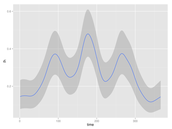
The number of occurrences of rainfall over 1 mm in the Tokyo area for each calendar year during two years (1983-84) are registered. It is of interest to estimate the underlying probability ${p_t}$ of rainfall for calendar day ${t}$ which is, a priori, assumed to change gradually over time. For each day ${t = 1, ..., 366}$ of the year we have the number of days that rained ${y_t}$ and the number of days that were observed ${n_t}$ . The model is given by

First stage: A conditionally independent binomial likelihood function
$\displaystyle y_t|\eta_t \sim \text{Bin}(n_t, p_t),\ t = 1, ..., 366$

with logit link function

$\displaystyle p_t = \frac{\exp(\eta_t)}{1 + \exp(\eta_t)}$
Second stage: We assume that ${\eta_t = f_t}$ , where ${f_t}$ follows a circular random walk 2 (RW2) model with precision ${\tau}$ . The RW2 model is defined by
$\displaystyle \Delta^2f_i = f_i - 2 f_{i+1} + f_{i+2} \sim N(0,\tau^{-1}).$

The fact that we use a circular model here means that in this case, ${f_1}$ is a neighbor of ${f_{366}}$ , since it makes sense to assume that the last day of the year has a similar effect when compared with the first day. So, in this case ${x = (f_1, ..., f_{366})}$ and again ${x|\theta}$ is Gaussian distributed.
Third stage: ${\theta = (\tau)}$ , where
$\displaystyle \tau \sim \text{gamma}(c_1, c_2)$

Here you can find the data and INLA code to fit this model, and below is the posterior mean of ${p_t}$ together with ${95\%}$ credible interval.

Disease mapping in Germany

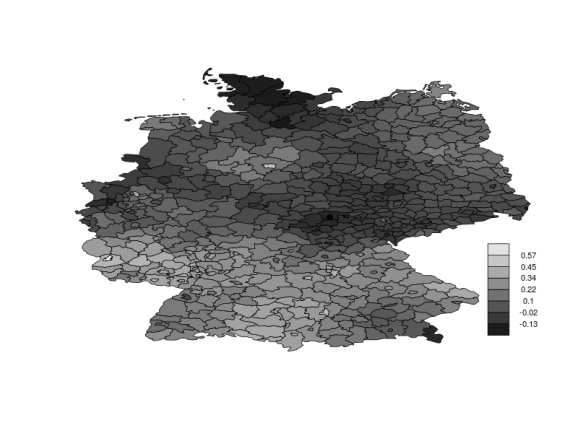
Larynx cancer mortality counts are observed in the 544 district of Germany from 1986 to 1990. Together with the counts, for each district, the level of smoking consumption c is registered. The model is given by

First stage: We assume the data to be conditionally independent Poisson random variables with mean ${E_i\exp(\eta_i)}$ , where ${E_i}$ is fixed and accounts for demographic variation, and ${\eta_i}$ is the log-relative risk.
$\displaystyle y_i|\eta_i \sim \text{Poisson}(E_i\exp(\eta_i)),\ i = 1, ..., 544$
Second stage: The linear predictor ${\eta_i}$ is formed by an intercept ${\mu}$ , an smooth function of the smoking consumption covariate ${f(c_i)}$ , an spatial model over different district locations ${f_s(s_i)}$ , and an unstructured random effect ${u_i}$ to account for overdispersion. So that
$\displaystyle \eta_i = \mu + f_s(s_i) + f(c_i) + u_i$

and the detailed description of each of the above model components can be found here. But again (surprise surprise) ${x|\theta}$ is Gaussian distributed.
Third stage: ${\theta}$ is formed by the precision parameters associated with the smooth model for the covariate ${f(c_i)}$ , the spatial model ${f_s(s_i)}$ and the random effect ${u_i}$ , all of which we assign gamma priors.

Here you can find the data and INLA code to fit this model, and below is the posterior mean of the spatial effect in each of the 544 districts in Germany.

Further reading:

– Examples and tutorials page in the INLA website.

– Slides of a Bayesian computation with INLA short-course I gave in the AS2013 conference in Ribno, Slovenia.

To leave a comment for the author, please follow the link and comment on their blog: Thiago G. Martins » R.

R-bloggers.com offers daily e-mail updates about R news and tutorials about learning R and many other topics. Click here if you're looking to post or find an R/data-science job.

Want to share your content on R-bloggers? click here if you have a blog, or here if you don't.

R-bloggers

R news and tutorials contributed by hundreds of R bloggers

Latent Gaussian Models and INLA

Related

Related

Never miss an update! Subscribe to R-bloggers to receive e-mails with the latest R posts. (You will not see this message again.)

Never miss an update!
Subscribe to R-bloggers to receive
e-mails with the latest R posts.
(You will not see this message again.)