In classical linear modelling we are assuming that the response variable (Y) is normally distributed, however for certain type of data like count data or presence/absence data this is not the case.

There is in statistic an ensemble of technique called Generalized Linear Modelling (GLM in short) where the reponse variable follow one known distribution, these are for example: gaussian, poisson, Bernoulli or binomial.

A GLM is made of three parts: the assumptions of the distribution of the response variable, the predictors used to build the model (the X part) and the link between the predictors and the response variable.

Let’s first see an exmple of GLM with a gaussian distribution (which is basically a linear model)

#load the dataset airquality measuring various climatic variables
 data(airquality)
 m_glm1<-glm(Temp~Wind,airquality,family="gaussian")
 m_lm<-lm(Temp~Wind,airquality)

#you can compare the two output which gives similar estimates of the slope and intercept
 summary(lm)
 summary(glm)

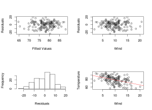
#model validation plot, residuals vs fitted values, residuals vs predictors and histogramm of #residuals
 r<-residuals(m_glm1)
 f<-fitted.values(m_glm1)
 par(mfrow=c(2,2))
 plot(r~f)
 plot(r~airquality$Wind)
 hist(r)

#add a plot with the estimated intercept and slope (which are both significantly different from #0)
 plot(Temp~Wind,airquality)
 abline(a=90.1349,b=-1.2305,col="red")

From this example we see that linear models are GLM with a gaussian distribution. The model validation plot show that there is no pattern in the residuals which could violate the assumption of the homogeneity of the variance and the residuals are normally distributed. The conclusion that we can draw from this are: the wind values significantly affect the temperature value in a negative way.

Know let’s look at some data which are not normally distributed, count data which follow a poisson distribution:

#a poisson example with the count of Amphibians road kills (Zuur, 2009)
rk<-data.frame(death=c(22,14,65,55,88,104,49, 66, 26, 47, 35, 55, 44, 30, 33, 29, 34, 64, 76, 32, 34, 32, 35, 22, 34, 25, 18,14, 14, 7, 7, 17, 10, 3, 6, 5, 2, 3, 2, 2, 7, 3, 5, 4, 7, 12, 7, 14, 10, 4, 11, 3)
,distance=250.214 , 741.179, 1240.080, 1739.885, 2232.130, 2724.089, 3215.511, 3709.401, 4206.477, 4704.176,5202.328, 5700.669, 6199.342, 6698.151, 7187.762, 7668.833, 8152.155, 8633.224, 
9101.411, 9573.578,10047.630, 10523.939, 11002.496, 11482.896, 11976.232, 12470.968, 12968.285, 13465.914, 13961.321, 14432.954,14904.995, 15377.983, 15854.389, 16335.936, 16810.109, 
17235.045, 17673.064, 18167.269, 18656.949, 19149.507,19645.717, 20141.987, 20640.729, 21138.903, 21631.542, 22119.102 ,22613.647, 23113.450, 23606.088, 24046.886,24444.874, 24884.803)

#do a poisson model
m_glm2<-glm(death~distance,rk,family="poisson")
summary(m_glm2)

#model validation plot with the fitted data
r<-resid(m_glm2)
f<-fitted.values(m_glm2)
par(mfrow=c(2,2))
plot(r~f,ylab="Residuals",xlab="Fitted values")
plot(r~rk$distance,xlab="Distance",ylab="Residuals")
hist(r,main="",xlab="Residuals")
plot(death~distance,rk)

#add the predicted values with the 95% confidence interval
pred<-predict(m_glm2,type="response",se.fit=TRUE)
lines(rk$distance,pred$fit,lty=1,col="blue")
lines(rk$distance,pred$fit+1.96*pred$se.fit,lty=2,col="blue")
lines(rk$distance,pred$fit-1.96*pred$se.fit,lty=2,col="blue")

The summary command on a glm object give similar information as in a lm object. We have the formula call, informations about the distribution of the residuals, the estimated coefficiants; in this case they are on a logarithmic scale since the default link between the predictors and the response variable for a poisson distribution is the log function (see ?family). Then information on the total and residuals sum of squares, and an AIC coefficient which can be usefull when comparing different models.

Litterature:

Zuur et al books, http://highstat.com/books.htm

Zeilis et al, http://cran.r-project.org/web/packages/pscl/vignettes/countreg.pdf