Next on modelling survival data from Veterinary Epidemiologic Research: semi-parametric analyses. With non-parametric analyses, we could only evaluate the effect one or a small number of variables. To evaluate multiple explanatory variables, we analyze data with a proportional hazards model, the Cox regression. The functional form of the baseline hazard is not specified, which make the Cox model a semi-parametric model.
A Cox proportional hazards model is fit hereafter, on data from a clinical trial of the effect of prostaglandin adminsitration on the start of breeding period of dairy cows:

temp <- tempfile()
download.file(
"http://ic.upei.ca/ver/sites/ic.upei.ca.ver/files/ver2_data_R.zip", temp)
load(unz(temp, "ver2_data_R/pgtrial.rdata"))
unlink(temp)

library(Hmisc)
pgtrial <- upData(pgtrial, labels = c(herd = 'Herd id', cow = 'Cow id',
                             tx = 'Treatment', lact = 'Lactation number',
                             thin = 'Body condition', dar = 'Days at risk',
                             preg = 'Pregnant or censored'),
                  levels = list(thin = list('normal' = 0, 'thin' = 1),
                    preg = list('censored' = 0, 'pregnant' = 1)))
pgtrial$herd <- as.factor(pgtrial$herd)

library(survival)
coxph.mod <- coxph(Surv(dar, preg == 'pregnant') ~ herd + tx + lact + thin,
                   data = pgtrial, ties = 'breslow')
(coxph.sum <- summary(coxph.mod))
Call:
coxph(formula = Surv(dar, preg == "pregnant") ~ herd + tx + lact + 
    thin, data = pgtrial, ties = "breslow")

  n= 319, number of events= 264 

             coef exp(coef) se(coef)      z Pr(>|z|)  
herd2    -0.28445   0.75243  0.16981 -1.675   0.0939 .
herd3     0.03676   1.03744  0.17426  0.211   0.8329  
tx        0.18359   1.20152  0.12543  1.464   0.1433  
lact     -0.04283   0.95807  0.04109 -1.042   0.2972  
thinthin -0.14557   0.86453  0.13794 -1.055   0.2913  
---
Signif. codes:  0 ‘***’ 0.001 ‘**’ 0.01 ‘*’ 0.05 ‘.’ 0.1 ‘ ’ 1

         exp(coef) exp(-coef) lower .95 upper .95
herd2       0.7524     1.3290    0.5394     1.050
herd3       1.0374     0.9639    0.7373     1.460
tx          1.2015     0.8323    0.9396     1.536
lact        0.9581     1.0438    0.8839     1.038
thinthin    0.8645     1.1567    0.6597     1.133

Concordance= 0.564  (se = 0.021 )
Rsquare= 0.029   (max possible= 1 )
Likelihood ratio test= 9.5  on 5 df,   p=0.09084
Wald test            = 9.32  on 5 df,   p=0.09685
Score (logrank) test = 9.34  on 5 df,   p=0.09611

R gives several options to control ties in case several events occurred at the same time: the Efron method (default in R), Breslow method (default in software like SAS or Stata), and the exact method. Breslow is the simplest and adequate if not too many ties in the dataset. Efron is closer to the exact approximation.

Stratified Cox Propotional Hazards Model

In a stratified Cox model, different baseline hazards are assumed across groups of subjects. The Cox model is modified to allow the control of a predictor which do not satisfy the proportional hazards (PH) assumption. We refit the above model by stratifying by herd and including a treatment by herd interaction:

scoxph.mod <- coxph(Surv(dar, preg == 'pregnant') ~ tx + tx*herd + lact + thin +
                    strata(herd), data = pgtrial, method = 'breslow')
summary(scoxph.mod)
Call:
coxph(formula = Surv(dar, preg == "pregnant") ~ tx + tx * herd + 
    lact + thin + strata(herd), data = pgtrial, method = "breslow")

  n= 319, number of events= 264 

             coef exp(coef) se(coef)      z Pr(>|z|)  
tx       -0.02160   0.97863  0.25528 -0.085   0.9326  
herd2          NA        NA  0.00000     NA       NA  
herd3          NA        NA  0.00000     NA       NA  
lact     -0.04600   0.95504  0.04065 -1.132   0.2578  
thinthin -0.13593   0.87291  0.13833 -0.983   0.3258  
tx:herd2 -0.05659   0.94498  0.33570 -0.169   0.8661  
tx:herd3  0.54494   1.72451  0.31823  1.712   0.0868 .
---
Signif. codes:  0 ‘***’ 0.001 ‘**’ 0.01 ‘*’ 0.05 ‘.’ 0.1 ‘ ’ 1

         exp(coef) exp(-coef) lower .95 upper .95
tx          0.9786     1.0218    0.5934     1.614
herd2           NA         NA        NA        NA
herd3           NA         NA        NA        NA
lact        0.9550     1.0471    0.8819     1.034
thinthin    0.8729     1.1456    0.6656     1.145
tx:herd2    0.9450     1.0582    0.4894     1.825
tx:herd3    1.7245     0.5799    0.9242     3.218

Concordance= 0.56  (se = 0.035 )
Rsquare= 0.032   (max possible= 0.998 )
Likelihood ratio test= 10.32  on 5 df,   p=0.06658
Wald test            = 10.5  on 5 df,   p=0.0623
Score (logrank) test = 10.66  on 5 df,   p=0.05851

Evaluating the Assumption of Proportional Hazards

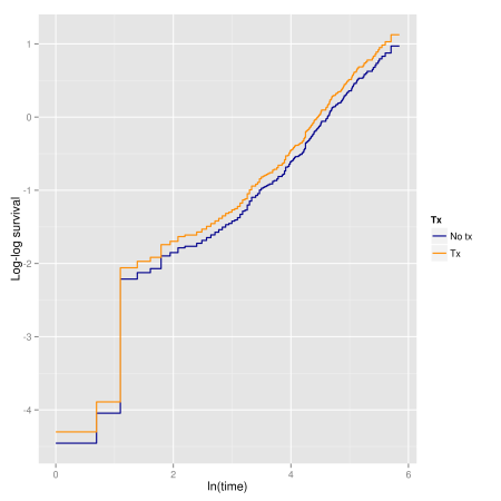
We can evaluate it graphically, by examining the log-cumulative hazard plot vs. ln(time) and check if the curves are parallel:

coxph.mod2 <- coxph(Surv(dar, preg == 'pregnant') ~ tx, data = pgtrial,
                   ties = 'breslow')
pgtrial2 <- with(pgtrial, data.frame(tx = c(0, 1)))
tfit.add <- survfit(coxph.mod2, newdata = pgtrial2)
df1 <- data.frame(
    time    = tfit.add[1, ]$time,
    n.risk  = tfit.add[1, ]$n.risk,
    n.event = tfit.add[1, ]$n.event,
    surv    = tfit.add[1, ]$surv,
    strata  = "0",
    upper   = tfit.add[1, ]$upper,
    lower   = tfit.add[1, ]$lower,
    log.surv = log(-log(tfit.add[1, ]$surv))
 ) 
df2 <- data.frame(
    time    = tfit.add[2, ]$time,
    n.risk  = tfit.add[2, ]$n.risk,
    n.event = tfit.add[2, ]$n.event,
    surv    = tfit.add[2, ]$surv,
    strata  = "1",
    upper   = tfit.add[2, ]$upper,
    lower   = tfit.add[2, ]$lower,
    log.surv = log(-log(tfit.add[2, ]$surv))
 )
dfpar.add <- rbind(df1, df2)
zeros <- data.frame(time = 0, surv = 1, strata = c(1, 2), 
                     upper = 1, lower = 1)
dfpar.add <- rbind.fill(zeros, dfpar.add)
dfpar.add$strata <- factor(dfpar.add$strata, labels = c("No tx", "Tx"))
ggplot(dfpar.add, aes(log(time), log.surv, colour = strata)) + 
  geom_step(size = 0.6) + 
  scale_color_manual("Tx", values = c('blue4', 'darkorange')) + 
  xlab("ln(time)") + ylab("Log-log survival")

Log cumulative hazard plot

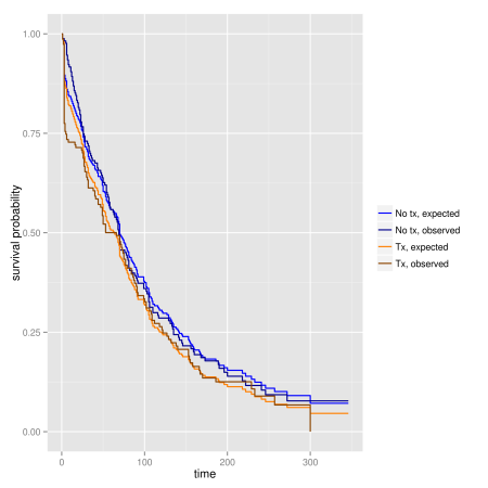
Another graphical approach is to compare plots of predicted survival times from a Cox model (assuming PH) to Kaplan-Meier survivor function (which do not assume PH):

tfit.km <- survfit(Surv(dar, preg == 'pregnant') ~ tx, data = pgtrial)
df3.km <- data.frame(
    time    = tfit.km$time,
    n.risk  = tfit.km$n.risk,
    n.event = tfit.km$n.event,
    surv    = tfit.km$surv,
    strata  = gsub("tx=", "", summary(tfit.km, censored = T)$strata),
    upper   = tfit.km$upper,
    lower   = tfit.km$lower
 ) 
zeros <- data.frame(time = 0, surv = 1, strata = gsub("tx=", "", 
                                          levels(summary(tfit.km)$strata)), 
                     upper = 1, lower = 1)
df3.km <- rbind.fill(df3.km, zeros)
df3.km$cat <- with(df3.km, ifelse(strata == "0", "No tx, observed",
                                  "Tx, observed"))
dfpar.add$cat <- with(dfpar.add, ifelse(strata == "No tx", "No tx, expected",
                                        "Tx, expected"))
dfpar.obs <- rbind.fill(dfpar.add, df3.km)
ggplot(dfpar.obs, aes(time, surv, colour = cat)) + 
   geom_step(size = 0.6) + 
   scale_color_manual("", values = c('blue1', 'blue4', 'darkorange1',
                            'darkorange4')) + 
   xlab("time") + ylab("survival probability")

Kaplan-Meier Cox plot

You can also assess PH statistically with the Schoenfeld residuals using cox.zph function:

(schoen <- cox.zph(coxph.mod))
             rho chisq      p
herd2    -0.0630 1.100 0.2942
herd3    -0.0443 0.569 0.4506
tx       -0.1078 3.141 0.0763
lact      0.0377 0.447 0.5035
thinthin -0.0844 2.012 0.1560
GLOBAL        NA 7.631 0.1778

plot(schoen, var = 4)

Schoenfeld residuals for lactation

Evaluating the Overall Fit of the Model

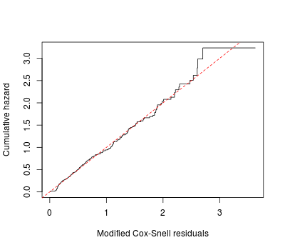
First we can look at the Cox-Snell residuals, which are the estimated cumulative hazards for individuals at their failure (or censoring) times. The default residuals of coxph in R are the martingale residuals, not the Cox-Snell. But it can be computed:

cox.snell <- (as.numeric(pgtrial$preg) - 1) - resid(coxph.mod,
                                                    type = "martingale")
coxph.res <- survfit(coxph(Surv(cox.snell, pgtrial$preg == 'pregnant') ~ 1,
                           method = 'breslow'), type = 'aalen')

plot(coxph.res$time, -log(coxph.res$surv), type = 's',
     xlab = 'Modified Cox-Snell residuals', ylab = 'Cumulative hazard')
abline(0, 1, col = 'red', lty = 2)

## Alternatively:
coxph.res2 <- survfit(Surv(cox.snell, pgtrial$preg == 'pregnant') ~ 1)
Htilde <- cumsum(coxph.res2$n.event / coxph.res$n.risk)
plot(coxph.res2$time, Htilde, type = 's', col = 'blue')
abline(0, 1, col = 'red', lty = 2)

Plot of Cox-Snell residuals

We can also use a goodness-of-fit test:

## GOF (Gronnesby and Borgan omnibus gof)
library(gof)
cumres(coxph.mod)

Kolmogorov-Smirnov-test: p-value=0.35
Cramer von Mises-test: p-value=0.506
Based on 1000 realizations. Cumulated residuals ordered by herd2-variable.
---
Kolmogorov-Smirnov-test: p-value=0.041
Cramer von Mises-test: p-value=0.589
Based on 1000 realizations. Cumulated residuals ordered by herd3-variable.
---
Kolmogorov-Smirnov-test: p-value=0
Cramer von Mises-test: p-value=0.071
Based on 1000 realizations. Cumulated residuals ordered by tx-variable.
---
Kolmogorov-Smirnov-test: p-value=0.728
Cramer von Mises-test: p-value=0.733
Based on 1000 realizations. Cumulated residuals ordered by lact-variable.
---
Kolmogorov-Smirnov-test: p-value=0.106
Cramer von Mises-test: p-value=0.091
Based on 1000 realizations. Cumulated residuals ordered by thinthin-variable.

We can evaluate the concordance between the predicted and observed sequence of pairs of events. Harrell’s c index computes the proportion of all pairs of subjects in which the model correctly predicts the sequence of events. It ranges from 0 to 1 with 0.5 for random predictions and 1 for a perfectly discriminating model. It is obtained from the Somer’s Dxy rank correlation:

library(rms)
fit.cph <- cph(Surv(dar, preg == 'pregnant') ~ herd + tx + lact + thin,
               data = pgtrial, x = TRUE, y = TRUE, surv = TRUE)
v <- validate(fit.cph, dxy = TRUE, B = 100)
Dxy <- v[rownames(v) == "Dxy", colnames(v) == "index.corrected"]
(Dxy / 2) + 0.5 # c index
[1] 0.4538712

Evaluating the Functional Form of Predictors

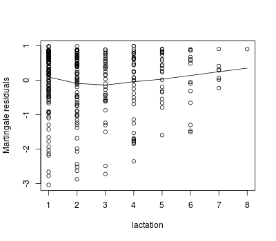
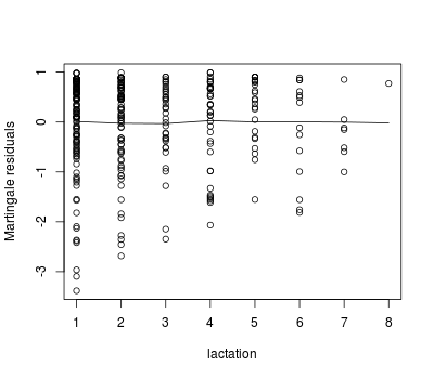
We can use martingale residuals to evaluate the functional form of the relationship between a continuous predictor and the survival expectation for individuals:

lact.mod <- coxph(Surv(dar, preg == 'pregnant') ~ lact, data = pgtrial,
                  ties = 'breslow')
lact.res <- resid(lact.mod, type = "martingale")
plot(pgtrial$lact, lact.res, xlab = 'lactation', ylab = 'Martingale residuals')
lines(lowess(pgtrial$lact, lact.res, iter = 0))
 
# adding quadratic term
lact.mod <- update(lact.mod, . ~ . + I(lact^2))
lact.res <- resid(lact.mod, type = "martingale")
plot(pgtrial$lact, lact.res, xlab = 'lactation', ylab = 'Martingale residuals')
lines(lowess(pgtrial$lact, lact.res, iter = 0))

Plot of marrtingale residuals vs. lactation number

Plot of martingale residuals vs. lactation number (as quadratic term)

Checking for Outliers

Deviance residuals can be used to identify outliers:

## deviance residuals
dev.res <- resid(coxph.mod, type = "deviance")
plot(pgtrial$dar, dev.res, xlab = 'time (days)', ylab = 'deviance residuals')

cbind(dev.res, pgtrial)[abs(dev.res) > 2, ]
      dev.res herd cow tx lact   thin dar     preg
1    2.557832    1   1  0    1 normal   1 pregnant
2    2.592492    1   2  1    4   thin   1 pregnant
3    2.319351    1   3  1    1 normal   2 pregnant
73  -2.693731    1  76  1    1 normal 277 censored
74   2.734508    2  78  0    2   thin   1 pregnant
75   2.644885    2  79  1    4 normal   1 pregnant
76   2.436308    2  80  1    1 normal   2 pregnant
176 -2.015925    2 180  1    2 normal 201 censored
180 -2.196008    2 184  1    2 normal 250 censored
183 -2.081493    2 187  1    3   thin 288 censored
185 -2.238729    2 189  0    1 normal 346 censored
314 -2.274912    3 318  0    1   thin 262 censored
315 -2.226711    3 319  0    2   thin 262 censored
316 -2.182517    3 320  0    4   thin 287 censored
317 -2.278029    3 321  0    2   thin 288 censored
318 -2.341736    3 322  0    3   thin 308 censored
319 -2.392427    3 323  0    2   thin 320 censored

Deviance residuals

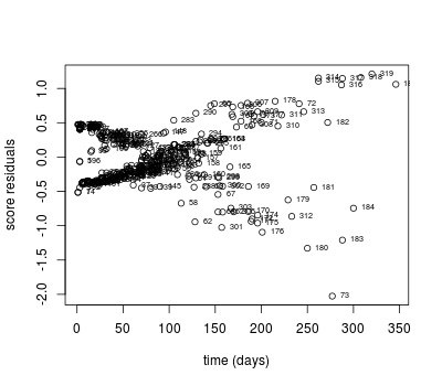
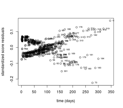
Score residuals and scaled score residuals can be used to identify influential observations:

### Detecting influential points
# score residuals
score.res <- resid(coxph.mod, type = "score")
# score residuals for tx
plot(pgtrial$dar, score.res[ , 3], xlab = 'time (days)',
     ylab = 'score residuals')
text(pgtrial$dar, score.res[ , 3], rownames(pgtrial), cex = 0.6, pos = 4)

cbind(score.res[ , 3], pgtrial)[abs(score.res[ , 3]) > 2, ]
   score.res[, 3] herd cow tx lact   thin dar     preg
73      -2.025537    1  76  1    1 normal 277 censored

## influential observations
dfbeta <- resid(coxph.mod, type = "dfbeta")
# dfbeta residuals for tx
plot(pgtrial$dar, dfbeta[ , 3], xlab = 'time (days)',
     ylab = 'scaled score residual')
text(pgtrial$dar, dfbeta[ , 3], rownames(pgtrial), cex = 0.6, pos = 4)

# with standardized dfbeta
dfbetas <- resid(coxph.mod, type = "dfbetas")
plot(pgtrial$dar, dfbetas[ , 3], xlab = 'time (days)',
     ylab = 'standardized score residuals')
text(pgtrial$dar, dfbetas[ , 3], rownames(pgtrial), cex = 0.6, pos = 4)

Score residuals

Scaled score residuals (delta-beta)

Standardized score residuals