I subscribe to the Ensembl blog and found, in my feed reader this morning, a post which linked to the Variant Effect Predictor (VEP). The original blog post, strangely, has disappeared.

Not to worry: so, the VEP takes genotyping data in one of several formats, compares it with the Ensembl variation + core databases and returns a summary of how the variants affect transcripts and regulatory regions. My first thought – can I apply this to my own 23andme data?

1. Convert 23andme data to VCF
If you download your raw data from 23andme, it looks something like this (ignoring comment lines):

rs4477212	1	82154	AA
rs3094315	1	752566	AA
rs3131972	1	752721	GG
rs12562034	1	768448	GG
rs12124819	1	776546	AA

The rest of this post assumes that your raw data are saved in a file named mySNPs.txt; note that the original file name of your download will be something like genome_YOUR_NAME_Full_TIMESTAMP.txt.zip.

VEP will accept several file formats, including VCF (variant call format). At Github, I discovered a tool named 23andme2vcf to perform the conversion. My first attempt failed:

perl 23andme2vcf.pl mySNPs.txt mySNPs.vcf
# raw data file and reference file are out of sync at ./23andme2vcf.pl line 154,  line 4.

Digging around the Github issues page, I noted that this error has occurred before; the issue was closed when the reference file supplied with 23andme2vcf was updated.

A quick line count reveals the problem: more SNPs in my 23andme data (V3 platform) than the reference file.

gunzip -c 23andme_hg19ref_20121017.txt.gz | wc -l
# 960613
grep -cv "^#" mySNPs.txt
# 991786

Easiest fix: read both into R, discard those SNPs not found in the reference file and write back out to a new tab-delimited file. To avoid discarding SNPs, you’ll have to figure out how to create the reference file; perhaps the issue will be fixed in a future update.

ref <- read.table("23andme_hg19ref_20121017.txt.gz", header = F, stringsAsFactors = F)
snp <- read.table("mySNPs.txt", header = F, stringsAsFactors = F)
snp <- subset(snp, V1 %in% ref$V3)
write.table(snp, "mynewSNPs.txt", quote = F, col.names = F, row.names = F, sep = "\t")

Now the conversion works as expected:

perl 23andme2vcf.pl mynewSNPs.txt mynewSNPs.vcf

Note that the script does not yet handle insertions or deletions. However, these are not well-defined in the 23andme data file in any case.

2. Install VEP locally
This is all as described in the VEP script documentation. Click the “download latest version” link, navigate to wherever you downloaded it and then:

tar zxvf variant_effect_predictor.tar.gz
cd variant_effect_predictor
perl INSTALL.pl

Follow the prompts. You will want to install the core and VEP files for Homo sapiens, the latest release being 71. Note that VEP files are a large download, currently ~ 2.5 GB, which will take some time.

3. Run VEP

From the variant_effect_predictor directory, as simple as:

perl variant_effect_predictor.pl --cache -i ~/path/to/mynewSNPs.vcf -o ~/path/to/myVEP.txt

Variant consequences from VEP

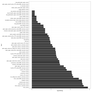
In addition to the delimited text output (mine is around 163 MB in size), the script generates a rather nice HTML summary with some statistics. It’s also easy to read the output from VEP back into R. See plot, right, for a summary of the VEP Consequence column.

library(ggplot2)
vep <- read.table("vep.txt", header = F, stringsAsFactors = F, sep = "\t")
colnames(vep) <- c("Uploaded_variation", "Location", "Allele",  "Gene", "Feature", "Feature_type",
                   "Consequence", "cDNA_position", "CDS_position", "Protein_position", "Amino_acids",
                   "Codons", "Existing_variation", "Extra")
cons <- as.data.frame(table(vep$Consequence))
cons <- cons[sort.list(cons$Freq, decreasing = T),]
cons$Var1 <- factor(cons$Var1, levels = cons$Var1)
ggplot(cons) + geom_bar(aes(Var1, log10(Freq)), stat = "identity") + coord_flip() + theme_bw()

It’s a lot of output to trawl through and summarize; I’ll post on the topic again if I discover anything interesting.