Still going through the book Veterinary Epidemiologic Research and today it’s chapter 18, modelling count and rate data. I’ll have a look at Poisson and negative binomial regressions in R.
We use count regression when the outcome we are measuring is a count of number of times an event occurs in an individual or group of individuals. We will use a dataset holding information on outbreaks of tuberculosis in dairy and beef cattle, cervids and bison in Canada between 1985 and 1994.

temp <- tempfile()
download.file(
"http://ic.upei.ca/ver/sites/ic.upei.ca.ver/files/ver2_data_R.zip",
temp)
load(unz(temp, "ver2_data_R/tb_real.rdata"))
unlink(temp)

library(Hmisc)
tb_real<- upData(tb_real, labels = c(farm_id = 'Farm identification',
                            type = 'Type of animal',
                            sex = 'Sex', age = 'Age category',
                            reactors = 'Number of pos/reactors in the group',
                            par = 'Animal days at risk in the group'),
                 levels = list(type = list('Dairy' = 1, 'Beef' = 2,
                                 'Cervid' = 3, 'Other' = 4),
                   sex = list('Female' = 0, 'Male' = 1),
                   age = list('0-12 mo' = 0, '12-24 mo' = 1, '>24 mo' = 2)))

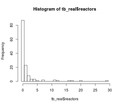
An histogram of the count of TB reactors is shown hereafter:

hist(tb_real$reactors, breaks = 0:30 - 0.5)

In a Poisson regression, the mean and variance are equal.

A Poisson regression model with type of animal, sex and age as predictors, and the time at risk is:

mod1 <- glm(reactors ~ type + sex + age + offset(log(par)), family = poisson, data = tb_real)
(mod1.sum <- summary(mod1))

Call:
glm(formula = reactors ~ type + sex + age + offset(log(par)), 
    family = poisson, data = tb_real)

Deviance Residuals: 
    Min       1Q   Median       3Q      Max  
-3.5386  -0.8607  -0.3364  -0.0429   8.7903  

Coefficients:
            Estimate Std. Error z value Pr(>|z|)    
(Intercept) -11.6899     0.7398 -15.802  < 2e-16 ***
typeBeef      0.4422     0.2364   1.871 0.061410 .  
typeCervid    1.0662     0.2334   4.569 4.91e-06 ***
typeOther     0.4384     0.6149   0.713 0.475898    
sexMale      -0.3619     0.1954  -1.852 0.064020 .  
age12-24 mo   2.6734     0.7217   3.704 0.000212 ***
age>24 mo     2.6012     0.7136   3.645 0.000267 ***
---
Signif. codes:  0 ‘***’ 0.001 ‘**’ 0.01 ‘*’ 0.05 ‘.’ 0.1 ‘ ’ 1 

(Dispersion parameter for poisson family taken to be 1)

    Null deviance: 409.03  on 133  degrees of freedom
Residual deviance: 348.35  on 127  degrees of freedom
AIC: 491.32

Number of Fisher Scoring iterations: 8

### here's an other way of writing the offset in the formula: 
mod1b <- glm(reactors ~ type + sex + age, offset = log(par), family = poisson, data = tb_real)

Quickly checking the overdispersion, the residual deviance should be equal to the residual degrees of freedom if the Poisson errors assumption is met. We have 348.4 on 127 degrees of freedom. The overdispersion present is due to the clustering of animals within herd, which was not taken into account.

The incidence rate and confidence interval can be obtained with:

cbind(exp(coef(mod1)), exp(confint(mod1)))
Waiting for profiling to be done...
                                2.5 %       97.5 %
(Intercept) 8.378225e-06 1.337987e-06 2.827146e-05
typeBeef    1.556151e+00 9.923864e-01 2.517873e+00
typeCervid  2.904441e+00 1.866320e+00 4.677376e+00
typeOther   1.550202e+00 3.670397e-01 4.459753e+00
sexMale     6.963636e-01 4.687998e-01 1.010750e+00
age12-24 mo 1.448939e+01 4.494706e+00 8.867766e+01
age>24 mo   1.347980e+01 4.284489e+00 8.171187e+01

As said in the post for logistic regression, the profile likelihood-based CI is preferable due to the Hauck-Donner effect (overestimation of the SE) (see also abstract by H. Stryhn at ISVEE X).

The deviance and Pearson goodness-of-fit test statistics can be done with:

# deviance gof
pchisq(deviance(mod1), df.residual(mod1), lower = FALSE)
[1] 1.630092e-22
#Pearson statistic
mod1.pearson <- residuals(mod1, type = "pearson")
1-pchisq(sum(mod1.pearson^2), mod1$df.residual)
[1] 0

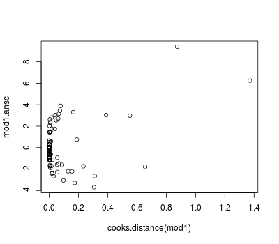
Diagnostics can be obtained as usual (see previous posts) but we can also use the Anscombe residuals:

library(wle)
mod1.ansc <- residualsAnscombe(tb_real$reactors, mod1$fitted.values, family = poisson())

plot(predict(mod1, type = "response"), mod1.ansc)
plot(cooks.distance(mod1), mod1.ansc)

Diagnostic plot – Anscombe residuals vs. predicted counts

Diagnostic plot – Anscombe residuals vs. Cook’s distance

Negative binomial regression models are for count data for which the variance is not constrained to equal the mean. We can refit the above model as a negative binomial model using full maximum likelihood estimation:

library(MASS)
mod2 <- glm.nb(reactors ~ type + sex + age + offset(log(par)), data = tb_real)
(mod2.sum <- summary(mod2))

Call:
glm.nb(formula = reactors ~ type + sex + age + offset(log(par)), 
    data = tb_real, init.theta = 0.5745887328, link = log)

Deviance Residuals: 
     Min        1Q    Median        3Q       Max  
-1.77667  -0.74441  -0.45509  -0.09632   2.70012  

Coefficients:
             Estimate Std. Error z value Pr(>|z|)    
(Intercept) -11.18145    0.92302 -12.114  < 2e-16 ***
typeBeef      0.60461    0.62282   0.971 0.331665    
typeCervid    0.66572    0.63176   1.054 0.291993    
typeOther     0.80003    0.96988   0.825 0.409442    
sexMale      -0.05748    0.38337  -0.150 0.880819    
age12-24 mo   2.25304    0.77915   2.892 0.003832 ** 
age>24 mo     2.48095    0.75283   3.296 0.000982 ***
---
Signif. codes:  0 ‘***’ 0.001 ‘**’ 0.01 ‘*’ 0.05 ‘.’ 0.1 ‘ ’ 1 

(Dispersion parameter for Negative Binomial(0.5746) family taken to be 1)

    Null deviance: 111.33  on 133  degrees of freedom
Residual deviance:  99.36  on 127  degrees of freedom
AIC: 331.47

Number of Fisher Scoring iterations: 1


              Theta:  0.575 
          Std. Err.:  0.143 

 2 x log-likelihood:  -315.472 

### to use a specific value for the link parameter (2 for example):
mod2b <- glm(reactors ~ type + sex + age + offset(log(par)),
             family = negative.binomial(2), data = tb_real)