PCA to PLS modeling analysis strategy for WIDE DATA

Working with wide data is already hard enough, add to this row outliers and things can get murky fast.

Here is an example of an anlysis of a wide data set, 24 rows  x 84 columns.

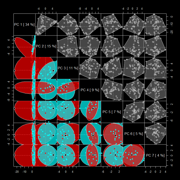
Using imDEV, written in R, to calculate and visualize a principal components analysis (PCA) on this data set. We find that 7 components capture >80% of the variance in the data or X. We can  also clearly see that the first dimension, capturing 35% of the variance in X, is skewed towards one outlier,  larger black point in the plots in the lower left triangle of the figure below, representing PCA scores.

In this plot representing the results from a PCA:

• Bottom left triangle  = PCA SCORES,  red and cyan ellipses display 2 groups, outlier is marked by a larger black point
• Diagonal = PCA Eigen values or variance in X explained by the component
• Top right triangle = PCA Loadings, representing linear combinations variable weights  to reconstruct Sample scores

In actuality the large variance in the outlier is due to a single value imputation used to back fill missing values in 40% of the columns (variable) for this row (sample).

Removing this sample (and another more moderate outlier) and using partial least squares projection to latent structures discriminant analysis or PLS-DA to generate a projection of  X which maximizes its covariance with Y which here is sample membership among the two groups noted by point  and ellipse color  (red = group 1, cyan = group 2).

The PLS scores separation for the two groups is largely captured in the first latent variable (LV1, x-axis). However we can’t be sure that this separation is better than random chance. To test this we can generate permuted NULL models by using our original X data to discriminate between randomly permuted sample group assignments (Y). When doing the random assignments we can optionally conserve the proportion of cases in each group or maintain this at 1:1.

Comparing our models (vertical hashed line) cross-validated fit to the training data , Q^2, to 100 randomly permuted models (TOP PANEL above, cyan distribution), we see that generally our “one” model is better fit than that achieved for the random data. Another interesting parameter is the comparison of our model’s root mean error of prediction, RMSEP, or out of sample error to the  permuted models’ (BOTTOM PANEL above, dark green distribution).

To have more confidence in the assessment of our model we can conduct training and testing validations. We can do this by randomly splitting our original X data into 2/3 training and 1/3 test sets. By using the training data to fit the model, and then using this to predict group memberships for the test data we can get an idea of the model’s out of sample classification error, visualized below using an receiver operator characteristic curve (ROC, RIGHT PANEL).

Wow this one model looks “perfect”, based on its assessment using one training/testing evaluation (ROC curve above). However it is important to repeat this procedure to evaluate its performance for other random splits of the data into training and test sets.

After permuting the samples training/test assignments 100 times; now we see that our original “one” model (cyan line in ROC curve in the TOP PANEL) was overly optimistic compared to the average performance of 100 models (green lines and distribution above).

Now that we have more confidence in our models performance we can compare the distributions for its performance metrics to those we calculated for the permuted NULL models above. In the case of the “one” model we can use a single sample t-Test or for the “100″ model a two-sample t-Test to determine the probability of achieving a similar performance to our model by random chance.

Now by looking at our models RMSEP compared to random chance (BOTTOM LEFT PANEL, out of sample error for our model, green, compared to random chance, yellow) we can be confident that our model is worth exploring further.

For example, we can now investigate the variables’ weights and loadings in the  PLS model to understand key differences in these parameters which are driving the above models discrimination  performance of our two groups of interest.