Partial least squares projection to latent structures or PLS is one of my favorite modeling algorithms.

PLS is an optimal algorithm for predictive modeling using wide data or data with  rows << variables. While there is s a wealth of literature regarding the application of PLS to various tasks, I find it especially useful for biological data which is often very wide and comprised of heavily inter-correlated parameters. In this context PLS is useful for generating  single dimensional answers  for multidimensional or multi factorial questions while overcoming the masking effects of redundant information or multicollinearity.

In my opinion an optimal PLS-based classification/discrimination model (PLS-DA) should capture the maximum difference between groups/classes being classified in the first dimension or latent variable (LV) and all information orthogonal to group discrimination should omitted from the model.

Unfortunately this is almost never the case and typically the plane of separation between class scores  in PLS-DA models span two or more dimensions. This is sub-optimal because we are then forced to consider more than one dimension or model latent variable (LV) when answering the question: how are variables the same/different between classes and which of  differences are the most important.

To the left is an example figure showing how principal components (PCA), PLS-DA and orthogonal PLS-DA (OPLS-DA) vary in their ability to capture the maximum variance between classes (red and cyan) in the first dimension or LV (x-axis).

Both OPLS and orthogonal signal correction-PLS (OSC-PLS) aim to maximize the captured variance between in the first dimension (x-axis).

Unfortunately there are no user friendly functions in R for carrying out OPLS or OSC-PLS. Note-  the package muma contains functions for OPLS, but it is not easy to use because it is deeply embedded within an automated reporting scheme.

Luckily Ron Wehrens published an excellent book titled Chemometrics with R which contains an R code example for carrying out OSC-PLS in a manner similar to the goal of OPLS.

I adapted his code  to make some user friendly functions (see below) for generating OSC-PLS models and plotting their results . I then used these to generate PLS-DA and OSC-PLS-DA models for a human glycomics data set. Lastly I compare OSC-PLS-DA and OPLS-DA (calculated using SIMCA 13) model scores.

The first task is to calculate a large (10 LV) exploratory model for 0 and 1 OSC-LVs.

Doing this we see that a 2 component model minimize the root mean squared error of prediction on the training data (RMSEP), and the OSC-PLS-DA model has a lower error than PLS-DA. Based on this we can calculate and compare the sample scores, variable loadings, and changes in model weights for 0 and 1 OSC PLS-DA models.

Comparing model (sample/row) scores between PLS-DA (0 OSC) and OSC-PLS-DA (1 OSC) models we can see that the OSC-PLS-DA model did a better job of capturing the maximal separation between the two sample classes (0 and 1) in the first dimension (x-axis).

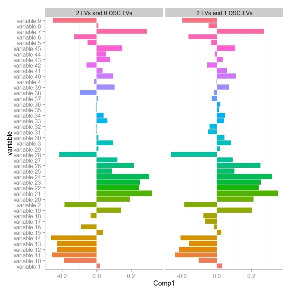
Next we can look at how model variable loadings for the 1st LV are different between the PLS-DA and OSC-PLS-DA models.

We can see that for the majority of variables the magnitude for the model loading was not changed much however there were some parameters whose sign for the loading changed (example: variable 8). If we we want to use the loadings in the 1st LV to encode the variables importance for discriminating between classes in some other visualization (e.g. to color and size nodes in a model network)  we need to make sure that the sign of the variable loading accurately reflects each parameters relative change between classes.

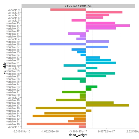
To specifically focus on how OSC effects the models perception of variables importance or weights we can calculate the differences in weights (delta weights ) between PLS-DA and OSC-PLS-DA models.

Comparing changes in weights we see that there looks to be a random distribution of increases or decreases in weight. variables 17 and 44 were the most increased in weight post OSC and 10 and 38 most decreased. Next we probably would want to look at the change in weight relative to the absolute weight (not shown).

Finally I wanted to compare OSC-PLS-DA  and OPLS-DA model scores. I used Simca 13 to calculate the OPLS-DA model parameters and then devium and inkcape to make a scores visualization.

Generally PLS-DA and OPLS-DA show a similar degree of class separation in the 1st LV. I was happy to see that the OSC-PLS-DA model seems to have the largest class scores resolution and likely the best predictive performance of all three algorithms, but I will need to validate this by doing model permutations and  training and testing evaluations.

Check out the R code  used for this example  HERE.