Update March 5th
All downloads are now accessible from my script page!

Summary
This posting shows how to plot frequency plots using the ggplot-package in R. Compared to SPSS standard outputs, you will learn how to create appealing diagrams ready for use in your papers.

Frequency plots in SPSS
In SPSS, you can create frequencies of variables by using this short script:

FREQUENCIES VARIABLES=c96cop15   /ORDER=ANALYSIS.

which gives you following overview:

If you add another line to your syntax script, you can plot either bar charts (/BARCHARTS) or histograms (/HIST), too:

FREQUENCIES VARIABLES=c96cop15   /ORDER=ANALYSIS.   /BARCHART FREQ

which gives you following results:

SPSS Bar Chart

SPSS Histrogram

It seems to be more effort creating graphs like the ones above in R, but actually it’s almost easier – and you even have more beautiful plots. The only preparation you need is a general function for plotting frequencies in R.

Frequency plots in R using ggplot
Honestly, writing such a function is an effort and takes some time. But once you’ve written it, you can use and reuse it for many situations with (almost) no further adjustments, in case you’ve made it flexible enough to meet your needs.

I will not explain this function in detail because it would take too much space in this posting. Furthermore, I added lots of comments to the script file which should help understanding the code. The R script-file sjPlotFrequencies.R can be downloaded here: script page.

The plotting function is called sjp.frq() and requires at least one parameter (the variable which category frequencies should be plotted). However, you can supply many additional parameters to manipulate the output style of your diagram.

You can change following characteristics via parameters (see header of R-file for more information):

• diagram title
• x-Axis and value Labels
• line wrap postion, when labels and title will break into a new line
• angle of x-axis-labels
• label color
• value label color
• diagram border color
• diagram background (theme)
• automatic calculation of maximum limit of the y-axis
• pre-defined limit of the y-axis
• when to use histogram or bar charts
• bar width
• bar color
• bar transparancy
• bar outline color
• whether value labels should be drawn or not
• whether outline should be drawn or not
• include NA’s or not
• …and more

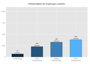
Here are some examples (refer to this posting to see how variables and labels have been imported from a SPSS dataset).

j <- 86 # variable index (column) number
sjp.frq(efc[,j],
        title = efc_vars[j],
        axisLabels.x = efc_label[[j]])

Or you can use the variable name instead of its column number.

sjp.frq(efc[,'e42dep'],
        title = efc_vars['e42dep'],
        axisLabels.x = efc_label[['e42dep']])

R frequency plot with ggplot, standard parameters

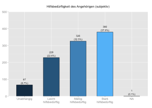
sjp.frq(efc[,j],
        title = efc_vars[j],
        axisLabels.x = efc_label[[j]],
        upperYlim = 500,
        omitNA = FALSE)

R frequency plot with ggplot, with NA’s included and y-axis-limit of 500

sjp.frq(efc[,j],
        upperYlim = 500,
        axisLabels.x = c("#cccccc"),
        outlineColor= c("#999999"))

R frequency plot with ggplot, no title and x-axis-lables, grey colored bars and outline

Variables with more than 10 categories will be plotted as histogram (you can change this breakpoint where automatically histrograms are plotted instead of bar charts with a parameter as well). If you want to plot histograms, use the type parameter. You can choose between three different types of histograms: bar charts, density plot with curve or filled area with line.

sjp.frq(efc$c160age, 
        title = efc_vars['c160age'], 
        type="hist",
        barOutline=TRUE,
        showMeanIntercept=TRUE)

Bar-chart-histogram with vertical mean intercept line

sjp.grp(efc$c160age, 
        title = efc_vars['c160age'], 
        type="d")

Histogram with density curve

sjp.frq(efc$c160age, 
        title = efc_vars['c160age'],   
        type="l")

Histogram with filled area and line curve

Another great thing is that you can easily plot a set of charts into a PDF file that contains scalable diagrams, i.e. high resolution ready-to-print graphics. The following code will create a PDF file with about 50 diagrams, containing both bar charts (variables with less than 10 categories) and histograms with density curve (variables with 10+ categories).

outputPDFPath <- c("/Users/danielludecke/Desktop/frequencies.pdf")
pdf(file=outputPDFPath)
from <- 291 # start first chart with variable (column) no. 291
to <- 343 # finish with variable (column) no. 343
for (j in from:to) {
  print(sjp.grp(gemo[,j],
          title = gemo_vars[j],
          axisLabels.x=gemo_label[[j]])
  print(to-j) # print progress to console
}
dev.off()

Final remarks
At least on my iMac, I can simply drag and drop single PDF pages containing the diagrams from the Preview app into Word – creating (scientific) graph almost the fastest way, with the help of R and ggplot.

If you look for more resources on how to improve your workflow, take a look at this posting in TRinker’s R Blog. Futhermore, R-Bloggers is always worth a visit…

Any comments, suggestions and tips on how to optimize my scripts are very welcome!