Chemical Reactor Analysis and Design Fundamentals by J.B. Rawlings and J. G. Ekerdt is a textbook for studying Chemical Reaction Engineering. The popular open source package Octave has its origins to the reaction engineering course offered by Prof. Rawlings. This book is accompanied by Octave and Matlab code for solving typical problems encountered in Reaction Engineering.

I figured that maybe one way to learn R is so see whether I can code some of th examples from this book in R. I am by no means suggesting that R can replace MATLAB/Octave for engineering problems but merely it is a way for me to learn the language.

I started with the computational appendix listed in the book’s website and am trying to work through some of the examples there. It will be good to refer to the computational appendix to follow the R code below.

# stoichiometric matrix
stoi=matrix(c(0,1,0,-1,-1,1,
-1,1,1,-1,0,0,
1,0,-1,0,-1,1),
ncol=6,byrow=T)
> stoi
[,1] [,2] [,3] [,4] [,5] [,6]
[1,]    0    1    0   -1   -1    1
[2,]   -1    1    1   -1    0    0
[3,]    1    0   -1    0   -1    1

# rank of the stoichiometrix matrix
rank=qr(stoi)$rank
> rank
[1] 2

# reaction rate vector
r=c(1,2,3)

Given the reaction rate r=(r1,r2)’, the rate of change of species concentration R is given by

where is the stoichiometrix matrix

# rate of change of components
R=t(stoi)%*%r
> R
[,1]
[1,]    1
[2,]    3
[3,]   -1
[4,]   -3
[5,]   -4
[6,]    4

Example A1: Estimating reaction rates

The stoichometrix matrix is input below

# stoichiometry
stoi=matrix(c(0,1,0,-1,-1,1,
-1,1,1,-1,0,0),nrow=2,byrow=T)
> stoi
[,1] [,2] [,3] [,4] [,5] [,6]
[1,]    0    1    0   -1   -1    1
[2,]   -1    1    1   -1    0    0

# number of species and number of reactions
nspec=ncol(stoi)
nr=nrow(stoi)

> nspec
[1] 6
> nr
[1] 2

# true rxn rates
r=c(1,2)
> r
[1] 1 2

# true component rates
R=t(stoi)%*%r
> R
[,1]
[1,]   -2
[2,]    3
[3,]    2
[4,]   -3
[5,]   -1
[6,]    1

Simulate 2000 measured component rates

Add random noise (normally distributed with mean 0 and standard deviation 0.05) to true species rate vector R

## simulate 2000 noise estimates
e=matrix(0.05*rnorm(2000*nspec,0,1),nrow=2000,byrow=T)
Rmeas=matrix(rep(R,2000),ncol=nspec,byrow=T)+e

The least squares estimate of reaction rate vector is

## estimate reaction rates
rest=solve(stoi%*%t(stoi),stoi%*%t(Rmeas))

I was trying different plot features in R and applying to this data of estimated rates.
I found the following function that plots scatterplot with marginal histograms

# plotting scatterplot with histogram
# downloaded from web
#  https://www.r-bloggers.com/example-8-41-scatterplot-with-marginal-histograms/
#
scatterhist = function(x, y, xlab="", ylab=""){
par.default <- par(no.readonly=TRUE)
zones=matrix(c(2,0,1,3), ncol=2, byrow=TRUE)
layout(zones, widths=c(4/5,1/5), heights=c(1/5,4/5))
xhist = hist(x, plot=FALSE)
yhist = hist(y, plot=FALSE)
top = max(c(xhist$counts, yhist$counts))
par(mar=c(3,3,1,1))
plot(x,y)
par(mar=c(0,3,1,1))
barplot(xhist$counts, axes=FALSE, ylim=c(0, top), space=0)
par(mar=c(3,0,1,1))
barplot(yhist$counts, axes=FALSE, xlim=c(0, top), space=0, horiz=TRUE)
par(oma=c(3,3,0,0))
mtext(xlab, side=1, line=1, outer=TRUE, adj=0,
at=0.9 * (mean(x) - min(x))/(max(x)-min(x)))
mtext(ylab, side=2, line=1, outer=TRUE, adj=0,
at=(0.9 * (mean(y) - min(y))/(max(y) - min(y))))
par=par(par.default)

}

# scatter plot of reaction rates with marginal histograms
scatterhist(t(rest)[,1],t(rest)[,2],xlab="r_1",ylab="r_2")

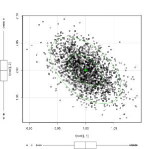
There is library cars that has a command ‘scatterplot’ for plotting scatterplot with box plots and has several other options
In the plot below 50% and 90% ellipses are overlaid on the data

# scatter plot of reaction rates with marginal box plots
library(car)
scatterplot(t(rest)[,1],t(rest)[,2],reg.line=FALSE,smooth=FALSE,ellipse=TRUE)

I tried ggplot2 also for the same plot

# 2d contours/density with ggplot2 for reaction rates

# create dataframe of reaction rates
rest_df=data.frame(t(rest))
names(rest_df)=c("r1","r2")

library(ggplot2)
ggplot(data=rest_df,aes(x=r1,y=r2))+geom_point()

ggplot(data=rest_df,aes(x=r1,y=r2))+stat_density2d()

ggplot(data=rest_df,aes(x=r1,y=r2))+stat_density2d(aes(fill=..level..),geom="polygon")