A nice, but not very well known, interface to R is
TeXmacs. (I have to say that I am not totally objective, since I wrote the interface between R and TeXmacs…)

Here’s a sample window:

In the following few posts I’d like to explain how to use this interface.

Installation

First, install TeXmacs. Best is to install the latest and greatest version of the svn, because that will include the latest changes of the interface with R, and in particular syntax highlighting. If you don’t install the latest version, you’ll probably only miss syntax highlighting. In that case it would probably be good to still install the latest version of the TeXmacs library for R.

Now that TeXmacs is installed, we can start it.
From the command line, just enter:

texmacs

A nice window will open:

I will not go into how to work with TeXmacs very much, just the R interface.

Still, a few hints might help.

Now let’s work with R. Select the little monitor icon, and chose “R”.

Type:
> 1:100
TeXmacs responds with the output from R:
 [1]  1  2  3  4  5  6  7  8  9 10 11 12 13 14 15 16 17 18 [19] 19 20 21 22 23 24 25 26 27 28 29 30 31 32 33 34 35 36 [37] 37 38 39 40 41 42 43 44 45 46 47 48 49 50 51 52 53 54 [55] 55 56 57 58 59 60 61 62 63 64 65 66 67 68 69 70 71 72 [73] 73 74 75 76 77 78 79 80 81 82 83 84 85 86 87 88 89 90 [91] 91 92 93 94 95 96 97 98 99 100
What is nice in using TeXmacs as an interface to R is that you can now move up to the previous line, edit it, and press enter again. The output will be replaced by The new output.

If you would like to enter multiple lines of text at once, press shift-enter, instead of enter. The input field will expend, and nothing will be sent to the R process. Once you are done, press enter. Here is an example:

You also see two additional features: syntax highlighting, and special background colors for input and output text. To turn on this coloring scheme, select the aptly named menu item Document→add package→Program→varsession.

BTW: If you prefer to invert the behaviour of enter and shift-enter, select the option multiline input as shown below:

Graphics

TeXmacs+R can also handle graphics.

Enter the following expression:
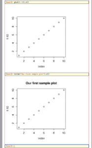
> plot(1:10);v()
Notice that after the first plot() command, usually a new window pops up, and you have to select the TeXmacs window again.
The result will look something like the following:

As you see, we needed two commands: the usual plot call, and v(). v() inserts the current plot as is into TeXmacs. So you can now do the following:
> title("Our first sample plot");v()
Which gives:

We now have a second copy of our graph, with a title. You could, of course, have done two plot commands and one v().
> plot(1:10);title("Our first sample plot");v()
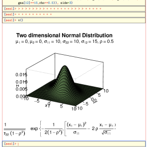
Let us try a more complicated example:
Here is a nice plot taken from the R Graph Gallery.

mu1mu2s11s12s22rhox1<-seq(-10,10,length=41) # generating the vector series x1
x2#
f<-function(x1,x2){
	term1 	term2 	term3 	term4 	term5 	term1*exp(term2*(term3+term4-term5))
} # setting up the function of the multivariate normal density
#
z<-outer(x1,x2,f) # calculating the density values
#
persp(x1, x2, z,
      main="Two dimensional Normal Distribution",
      sub=expression(italic(f)~(bold(x))==frac(1,2~pi~sqrt(sigma[11]~
                     sigma[22]~(1-rho^2)))~phantom(0)~exp~bgroup("{",
	             list(-frac(1,2(1-rho^2)),
	             bgroup("[", frac((x[1]~-~mu[1])^2, sigma[11])~-~2~rho~frac(x[1]~-~mu[1],
	             sqrt(sigma[11]))~ frac(x[2]~-~mu[2],sqrt(sigma[22])) ~+~
	             frac((x[2]~-~mu[2])^2, sigma[22]),"]")),"}")),
      col="lightgreen",
      theta=30, phi=20,
      r=50,
      d=0.1,
      expand=0.5,
      ltheta=90, lphi=180,
      shade=0.75,
      ticktype="detailed",
      nticks=5) # produces the 3-D plot
# adding a text line to the graph
mtext(expression(list(mu[1]==0,mu[2]==0,sigma[11]==10,sigma[22]==10,sigma[12]==15,rho==0.5)), side=3)

In order to paste this text properly into the R session, you will have to chose Edit→paste from→Verbatim. This is because TeXmacs normally treats the clipboard as representing a special TeXmacs format, not plain text.

One you press enter, you’ll see something like this:

At the Bottom you see a strange combination of > and +. These represent the prompts given by R as the lines are sent to the session. The current interface between TeXmacs and R can not tell when the R process finished evaluating its input. Not only that, but it might be that we’re not even finished with sending/receiving all the input lines. Thesefore, hit enter a couple more times, followed by v():

As you can see, the size of the graph doesn’t fit very well. We can control this by specifying the size of the image that should actually be produced by R v(width=8,height=8) (remember you can go up and edit the previous expression):

Much better!

Help

There are at least two ways of calling help in R inside TeXmacs. The first, is the usual help.start(), and using a web browser. The second, which is what I usually use, is to just ask for help in the usual way:

> ?plot
The help page is inserted formated into the current Buffer:

Working on a remote server

One of the best features of the TeXmacs+R interface is the ability to work on remote systems. To do that it is best to first set up a possibility for password-less ssh sessions (which means you need to ssh-keygen on the source system, and add the public key in the file ~/.ssh/authorized_hosts.)

You should also install the TeXmacs package on the remote system.

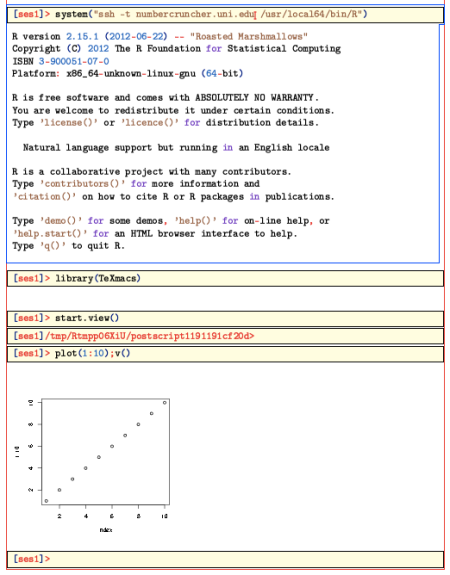
One that is set up, enter the following command in an R session:
> system("ssh -t REMOTE_HOST R")

You should then get the prompt of the remote system. (The argument ‘-t’ makes ssh open a ‘psydo-terminal’, which interacts better with TeXmacs) Now enter:
> library(TeXmacs)
And, if you’d like to use graphics,
> start.view()
This last command opens a postscript device, and sets it up so that the v() command will copy from it to TeXmacs.
Here is what things look like then:

Everything should work as on the local machine. Thus, you can ask R for help, and it should be inserted nicely formated into the current buffer.