I’ve started a tutorial on using the MODIS package in R the first few steps are here.  While I wait on a release of the package I thought I would play around a bit with the MRT tool and see how it worked.  Let’s recall where we are going.  I have an inventory of around 150 small cities and we are going to take a look at SUHI in those locations.  I have the DEM data, The Modis Land Class data, Olson Biomes, NLCD 30 meter land class and impervious surface. The last few bits I will need are MODIS LST and perhaps MODIS albedo ( If I get motivated) and EVI. We also have population data from a couple sources and housing data.

The first step to getting MODIS LST data is deciding what Tiles I need and then selecting dates. I had hoped that I might get away with using just a few tiles for the US, but that doesnt look like its going to happen. To figure out which Tiles I need there is a function in the MODIS package called getTile. But before I figured that out I tried to do it on my own. With some help from the geo sig list  I have the following to figure out the tiles.

First I get the  bounding coordinates for every tile

library(geosphere)

library(sp)

gring <-”http://landweb.nascom.nasa.gov/developers/sn_tiles/sn_gring_10deg.txt&#8221;

 
GRING <- read.table(gring, skip = 7, stringsAsFactors =FALSE, nrows=648,
na.strings=c(“-999.0000″,”-99.0000″))

colnames(GRING)<-c(“v”,”h”,”ll_lon”,”ll_lat”,
“ul_lon”,”ul_lat”,”ur_lon”,”ur_lat”,
“lr_lon”,”lr_lat”)

GRING <- GRING[!is.na(GRING[,3]),]

DF <- GRING[GRING$h < 15 & GRING$h > 6 & GRING$v < 7 & GRING$v > 3,]

The  table is downloaded and then I remove those rows that are NA. Next, I select those parts of the table that relate to CONUS  between  h(horizontal) 15 and 6 and vertical 7 and 3.

Next, I use Robert Hijmans code for generating a spatialpolygondataframe.

m <- as.matrix(DF)
z <- apply(m, 1, function(x) Polygon(matrix(x[c(3:10, 3:4)], ncol=2, byrow=T)))
n <- names(z)
y <- sapply(1:length(n), function(i) Polygons(z[i], n[i]))
sp <- SpatialPolygons(y, proj4string=CRS(‘+proj=longlat’))
spdf <- SpatialPolygonsDataFrame(sp, DF)

then we make some corrections for being on a sphere and we read in the lat/lon of all 150 sites
spdfc <- makePoly(spdf)

Inv <- read.table(“SiteInventory.inv”,stringsAsFactors = FALSE)

The next bit of clumsy code creates a spatial points data frame  that has 4 points for every site. I’m going to look +- .5degrees from the site center.

myExtent <- data.frame(lon=rep(NA,4*nrow(Inv)),lat=rep(NA,4*nrow(Inv)))

for( site in 1:nrow(Inv)){
dex <- ((site-1)*4)+1
myExtent$lon[dex]<- Inv$Lon[site] +.5
myExtent$lat[dex]<- Inv$Lat[site] -.5
myExtent$lon[dex+1]<- Inv$Lon[site] +.5
myExtent$lat[dex+1]<- Inv$Lat[site] +.5
myExtent$lon[dex+2]<- Inv$Lon[site] -.5
myExtent$lat[dex+2]<- Inv$Lat[site] -.5
myExtent$lon[dex+3]<- Inv$Lon[site] -.5
myExtent$lat[dex+3]<- Inv$Lat[site] +.5

}

Finally we will intersect the points with the SpatialPolygonsDataframe  and get out the tiles

pts <- SpatialPoints(myExtent)

proj4string(pts)<- proj4string(spdf)

Tiles <- over(pts,spdfc)[1:2]

Tiles <- unique(Tiles)

nrow( Tiles)

print(Tiles)

Depending on the increment I used  (.5 versus .2)  I basically had to collect 10-12 tiles to cover my bases for the next step.

With that list of tiles I downloaded the tiles I needed for  July4th  2006. In the future with the MODIS package this will happen just by writing code, but for now I did it by hand. With those 12 tiles downloaded I then fired up MRT to mosaic , resample, and reproject the tiles into a monolithic GeoTiff  for daytime LST for the whole Conus.

Reading that it we get the following

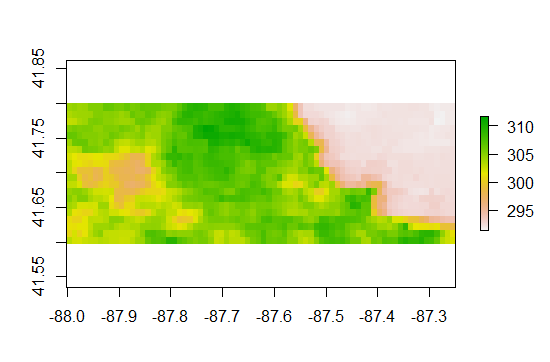
And then we can zoom in on the midwest and then go down chicago

On the left at  lon -87.9 lat 41.65  is the Paw Paw Woods Nature Preserve.  Pretty Cool