Dealing with endogeneity in a binary dependent variable model requires more consideration than the simpler continuous dependent variable case. For some, the best approach to this problem is to use the same methodology used in the continuous case, i.e. 2 stage least squares. Thus, the equation of interest becomes a linear probability model (LPM). The advantage of this approach is its simplicity; both in terms of estimation and interpretation (a 1-unit change in x causes a change in the probability of y).

The disadvantage of this approach is that the LPM may imply probabilities outside the unit interval. It is typically for this reason that generalized linear models, like probit or logit, are used to model binary dependent variables in applied research, and an approach that extends the probit model to account for endogeneity was proposed by Rivers & Vuong (1988).

The Rivers & Vuong estimator assumes the following usual triangular system:

(2),

wherein the jointly normally distributed error terms correlate, the control variables are in  and the instrumental variables are in . A simple procedure that estimates this model is the following two-step approach. First regress  on  and . Collect the residuals . The second step involves estimating the probit model of interest (2), and including the first stage residuals as an additional regressor. This method has also been termed the control function approach, as the inclusion of  controls for the correlation between  and .

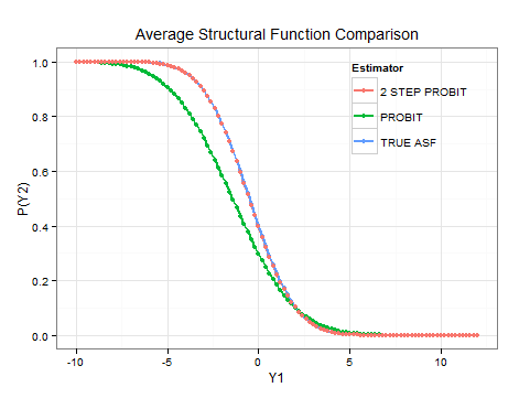
The second step coefficient estimates are scaled versions of their real values for reasons outlined here. It is possible to get the un-scaled values using the appropriate transformation. However, for analysis it is often more useful to know the Average Structural Function (ASF), as discussed in Blundell & Powell, 2004). The ASF can be seen as the policy response measure as it illustrates the probability of the dependent variable being a one given the values of the regressors, in the absence of endogeneity. Therefore, with the ASF it is possible to trace out the effects of changes in  on the probability of . Additionally, it is possible to compute average partial/marginal effects with the ASF, as described here.

Estimating the ASF involves taking the average of the normal CDF transformed predictions where the scaled coefficients are multiplied by all of the variables at some fixed value (commonly the mean) and all of the first-stage residuals are multiplied by the relevant scaled coefficient. This calculation is formalized on page 7 of this document.

To simulate the effect of changes in the endogenous variable, the ASF can be recursively estimated with different values of . I have attached an example of how this calculation can be performed for a simple simulation in R. It would also be possible to construct confidence intervals for this ASF using bootstrapping methods. As is evident from the plot, the control function estimator correctly identifies the ASF.

 
rm(list=ls())
library(mvtnorm)
n <- 10000
Sigma <- matrix(c(1,0.75,0.75,1),2,2)
u <- rmvnorm(n,rep(0,2),Sigma)

x1 <- rnorm(n)
x2 <- rnorm(n)
y1 <- 1.5 + 2*x1 - 2*x2 + u[,1] 
y2 <- ifelse(-0.25 - 1.25*x1 - 0.5*y1 + u[,2] > 0, 1, 0)

#true asf
eq1 <- function(x1,y1){pnorm(-0.25 - 1.25*x1 - 0.5*y1)}
data <- data.frame(cbind(mean(x1),seq(ceiling(min(y1)),floor(max(y1)),0.2)))
names(data) <- c("x1","y1")
data$asf <- eq1(data$x1,data$y1)

# naive probit: biased regression 
r1 <- glm(y2~x1+y1,binomial(link="probit"))
dat1 <- data.frame(cbind(mean(x1),seq(ceiling(min(y1)),floor(max(y1)),0.2)))
names(dat1) <- c("x1","y1")
asf1 <- cbind(dat1$y1,pnorm(predict(r1,dat1)))

# 2 step control function approach
v1 <- (residuals(lm(y1~x1+x2)))/sd(residuals(lm(y1~x1+x2)))
r2 <- glm(y2~x1+y1+v1,binomial(link="probit"))
# proceedure to get asf
asf2 <- cbind(seq(ceiling(min(y1)),floor(max(y1)),0.2),NA)
for(i in 1:dim(asf2)[1]){
  dat2 <- data.frame(cbind(mean(x1),asf2[i,1],v1))
  names(dat2) <- c("x1","y1","v1")
  asf2[i,2] <- mean(pnorm(predict(r2,dat2)))
  }

# get respective asfs and plot
plotdat <- data.frame(rbind(cbind(data$y1,data$asf,"TRUE ASF"),
                            cbind(data$y1,asf1[,2],"PROBIT"),
                            cbind(data$y1,asf2[,2],"2 STEP PROBIT")))
names(plotdat) <- c("Y1","Y2","Estimator")
plotdat$Y1 <- as.numeric(as.character(plotdat$Y1))
plotdat$Y2 <- as.numeric(as.character(plotdat$Y2))

library(ggplot2)
ggplot(plotdat, aes(x=Y1, y=Y2, colour = Estimator, group=Estimator)) + 
  geom_line(size=0.8) + geom_point()+
  scale_x_continuous('Y1') +
  scale_y_continuous('P(Y2)') +
  theme_bw() +
  opts(title = expression("Average Structural Function Comparison"),legend.position=c(0.8,0.8))