Network science is potentially useful for certain problems in data analysis, and I know close to nothing about it.

In this short post I present my first attempt at network analysis: A minimal example to construct and visualize an artificial undirected network with community structure in R. No network libraries are loaded. Only basic R-functions are used.

The final product of this post is this plot:

I am going to walk you through the code to produce the above plots. The complete code is given at the bottom of the post.

The starting point

First of all the network specification:

#network specs: K communities, N nodes, n[1] of them have 
#label 1, etc..., p(link inside)=p.in, p(link outside)=p.out
K     <- 3
N     <- 40 
n     <- c(rep(floor(N/K),K-1),floor(N/K)+N%%K)
labls <- rep(seq(K),n)
p.in  <- .9
p.out <- .1

pairs	   <- expand.grid(seq(N),seq(N))
uniq.pairs <- pairs[which(pairs[,1]<pairs[,2]),]
uniq.pairs <-lapply(apply(uniq.pairs,1,list),unlist) # I hate R for this line

There are N nodes and K communities. n[1] nodes are in community 1, n[2] in community 2, etc.

The probability p.in is the link probability between two nodes that are in the same community and p.out is the link probability across communities.

The variable labls contains the label of each node.

The variable pairs contains all possible tuples of the set (1,…,N). uniq.pairs is a list of 2-element vectors, containing only the unique links between nodes.

The p-matrix

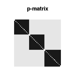
Such a network with community structure is typically modeled by what I would call a p-matrix (the technical term is “stochastic block matrix”). The entry in the i-th row and j-th column tells me the probability that node i is connected to node j. Since the network is undirected, a link between i and j is equivalent to a link between j and i, hence the p-matrix is symmetric. Furthermore no loops are allowed here, so the diagonal elements of the p-matrix are zero.

Community structure leads to the p-matrix being block-diagonal with large constant entries p.in in the blocks across the diagonal and small or vanishing entries p.out outside of these blocks.

#plot the block matrix
plot(NULL,xlim=c(1,N),ylim=c(1,N),asp=1,axes=F,xlab=NA,ylab=NA, main="p-matrix")
lapply( uniq.pairs, function(z) {
    colr <- ifelse(labls[z[1]]==labls[z[2]],gray(1-p.in), gray(1-p.out))
    points(z,N-z[c(2,1)],pch=15,col=colr) } )

The adjacency list

Based on the network specifications, an adjacency list is constructed. The adjacency list is the list of links in the network. A link between nodes i and j is realized with probability p.in if the nodes are in the same community, and with probability p.out otherwise.

#sample an adjacency list
adj.list   <- lapply(uniq.pairs,function(z) {
		p <- ifelse( labls[z[1]]==labls[z[2]],p.in,p.out)
		ifelse(runif(1)<p,1,0)*z})
adj.list   <- adj.list[ which(lapply(adj.list,sum)>0) ]

One way of visualizing the network is to plot the adjacency matrix which has dimension N*N and has a one at index (i,j) if nodes i and j are connected and a zero otherwise:

#plot the adjacency matrix
plot(NULL,xlim=c(1,N),ylim=c(1,N),asp=1,axes=F,xlab=NA,ylab=NA, main="adjacency matrix")
lapply( adj.list, function(z) {
    points(z,N-z[c(2,1)],pch=15) } )

Visualizing the links

Another way of visualizing the network is to plot the individual nodes and connect them with lines according to their links:

#plot the network
plot(NULL,xlim=c(0,K),ylim=c(0,1),axes=F,xlab=NA,ylab=NA, main="network")
coords <- matrix(runif(2*N),ncol=2)+cbind(labls-1,rep(0,N))
lapply( adj.list, function(z) {
         x <- coords[ z,1 ]
         y <- coords[ z,2 ]
         lines(x,y,col="#55555544") } )
colrs <- rainbow(K)
points( coords, pch=15, col=colrs[ labls ])

So far so good

This is it. As I said, it was the first step.

Next I want to look at ways to guess the node labels (the community structure) only based on the network structure, so stay tuned.

Thanks for watching.

———————-

The complete code:

######################################################
# construct and plot a stochastic block model, and a 
# corresponding network with community structure
######################################################

################################################################
#network specs: K communities, N nodes, n[1] of them have 
#label 1, etc..., p(link inside)=p.in, p(link outside)=p.out
################################################################
N     <- 40
K     <- 3
n     <- c(rep(floor(N/K),K-1),floor(N/K)+N%%K)
labls <- rep(seq(K),n)
p.in  <- .9
p.out <- .1

##############################################################
#sample an adjacency list
# pairs (uniq.pairs)  ... list of possible (unique) node pairs
# adj.list	      ... list of links between nodes
##############################################################
pairs	   <- expand.grid(seq(N),seq(N))
uniq.pairs <- pairs[which(pairs[,1]<pairs[,2]),]
uniq.pairs <-lapply(apply(uniq.pairs,1,list),unlist) # I hate R for this line
adj.list   <- lapply(uniq.pairs,function(z) {
		p <- ifelse( labls[z[1]]==labls[z[2]], p.in,p.out)
		ifelse(runif(1)<p,1,0)*z})
adj.list   <- adj.list[ which(lapply(adj.list,sum)>0) ]

#everything in one plot
jpeg("network.jpg",width=500,height=500,quality=100)
par(mar=c(2,2,4,2),cex.main=1.5)
layout(t(matrix(c(1,2,3,3),nrow=2)))

#plot the block matrix
plot(NULL,xlim=c(1,N),ylim=c(1,N),asp=1,axes=F,xlab=NA,ylab=NA, main="p-matrix")
lapply( uniq.pairs, function(z) {
    colr <- ifelse(labls[z[1]]==labls[z[2]],gray(1-p.in), gray(1-p.out))
    points(z,N-z[c(2,1)],pch=15,col=colr) } )

#plot the adjacency matrix
plot(NULL,xlim=c(1,N),ylim=c(1,N),asp=1,axes=F,xlab=NA,ylab=NA, main="adjacency matrix")
lapply( adj.list, function(z) {
    points(z,N-z[c(2,1)],pch=15) } )

#plot the network
plot(NULL,xlim=c(0,K),ylim=c(0,1),axes=F,xlab=NA,ylab=NA, main="network")
coords <- matrix(runif(2*N),ncol=2)+cbind(labls-1, rep(0,N))
lapply( adj.list, function(z) {
         x <- coords[ z,1 ]
         y <- coords[ z,2 ]
         lines(x,y,col="#55555544") } )
colrs <- rainbow(K)
points( coords, pch=15, col=colrs[ labls ])
dev.off()