Want to share your content on R-bloggers? click here if you have a blog, or here if you don't.
Typically, regression models in empirical economic research suffer from at least one form of endogeneity bias.
The classic example is economic returns to schooling, where researchers want to know how much increased levels of education affect income. Estimation using a simple linear model, regressing income on schooling, alongside a bunch of control variables, will typically not yield education’s true effect on income. The problem here is one of omitted variables – notably unobserved ability. People who are more educated may be more motivated or have other unobserved characteristics which simultaneously affect schooling and future lifetime earnings.
Endogeneity bias plagues empirical research. However, there are solutions, the most common being instrumental variables (IVs). Unfortunately, the exclusion restrictions needed to justify the use of traditional IV methodology may be impossible to find.
So, what if you have an interesting research question, some data, but endogeneity with no IVs. You should give up, right? Wrong. According to Lewbel (forthcoming in Journal of Business and Economic Statistics), it is possible to overcome the endogeneity problem without the use of a traditional IV approach.
Lewbel’s paper demonstrates how higher order moment restrictions can be used to tackle endogeneity in triangular systems. Without going into too much detail (interested readers can consult Lewbel’s paper), this method is like the traditional two-stage instrumental variable approach, except the first-stage exclusion restriction is generated by the control, or exogenous, variables which we know are heteroskedastic (interested practitioners can test for this in the usual way, i.e. a White test).
In the code below, I demonstrate how one could employ this approach in R using the GMM framework outlined by Lewbel. My code only relates to a simple example with one endogenous variable and two exogenous variables. However, it would be easy to modify this code depending on the model.
rm(list=ls())
library(gmm)
# gmm function for 1 endog variable with 2 hetero exogenous variable
# outcome in the first column of 'datmat', endog variable in second
# constant and exog variables in the next three
# hetero exog in the last two (i.e no constant)
g1 <- function(theta, datmat) {
  #set up data
  y1 <- matrix(datmat[,1],ncol=1)
  y2 <- matrix(datmat[,2],ncol=1)
  x1 <- matrix(datmat[,3:5],ncol=3)
  z1 <- matrix(datmat[,4:5],ncol=2)
  # if the variable in the 4th col was not hetero
  # this could be modified so:
  # z1 <- matrix(datmat[,5],ncol=1)

  #set up moment conditions
  in1 <- (y1 -theta[1]*x1[,1]-theta[2]*x1[,2]-theta[3]*x1[,3])
  M <- NULL
  for(i in 1:dim(z1)[2]){
    M <- cbind(M,(z1[,i]-mean(z1[,i])))
  }
  in2 <- (y2 -theta[4]*x1[,1]-theta[5]*x1[,2]-theta[6]*x1[,3]-theta[7]*y1)
  for(i in 1:dim(x1)[2]){M <- cbind(M,in1*x1[,i])}
  for(i in 1:dim(x1)[2]){M <- cbind(M,in2*x1[,i])}
  for(i in 1:dim(z1)[2]){M <- cbind(M,in2*((z1[,i]-mean(z1[,i]))*in1))}
  return(M)
}
# so estimation is easy
# gmm(function(...), data matrix, initial values vector)
# e.g : gmm(g1, x =as.matrix(dat),c(1,1,1,1,1,1,1))
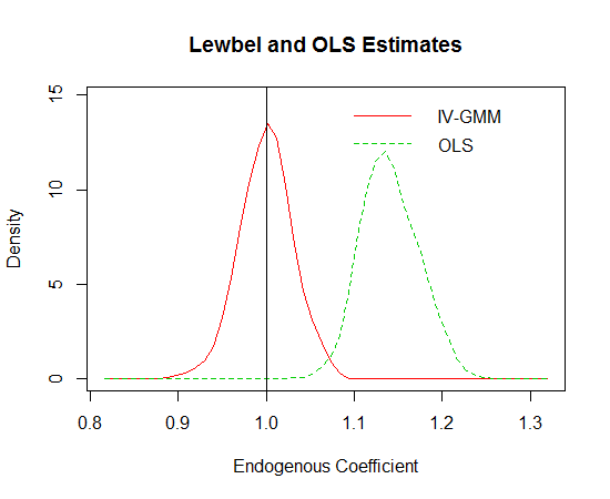
I also tested the performance of Lewbel’s GMM estimator in comparison a mis-specified OLS estimator. In the code below, I perform 500 simulations of a triangular system containing an omitted variable. For the GMM estimator, it is useful to have good initial starting values. In this simple example, I use the OLS coefficients. In more complicated settings, it is advisable to use the estimates from the 2SLS procedure outlined in Lewbel’s paper. The distributions of the coefficient estimates are shown in the plot below. The true value, indicated by the vertical line, is one. It is pretty evident that the Lewbel approach works very well. I think this method could be very useful in a number of research disciplines.
beta1 <- beta2 <- NULL
for(k in 1:500){
  #generate data (including intercept)
  x1 <- rnorm(1000,0,1)
  x2 <- rnorm(1000,0,1)
  u <- rnorm(1000,0,1)
  s1 <- rnorm(1000,0,1)
  s2 <- rnorm(1000,0,1)
  ov <- rnorm(1000,0,1)
  e1 <- u + exp(x1)*s1 + exp(x2)*s1
  e2 <- u + exp(-x1)*s2 + exp(-x2)*s2
  y1 <- 1 + x1 + x2 + ov + e2
  y2 <- 1 + x1 + x2 + y1 + 2*ov + e1
  x3 <- rep(1,1000)
  dat <- cbind(y1,y2,x3,x1,x2)

  #record ols estimate
  beta1 <- c(beta1,coef(lm(y2~x1+x2+y1))[4])
  #init values for iv-gmm
  init <- c(coef(lm(y2~x1+x2+y1)),coef(lm(y1~x1+x2)))
  #record gmm estimate
  beta2 <- c(beta2,coef(gmm(g1, x =as.matrix(dat),init))[7])
}

library(sm)
d <- data.frame(rbind(cbind(beta1,"OLS"),cbind(beta2,"IV-GMM")))
d$beta1 <- as.numeric(as.character(d$beta1))
sm.density.compare(d$beta1, d$V2,xlab=("Endogenous Coefficient"))
 title("Lewbel and OLS Estimates")
 legend("topright", levels(d$V2),lty=c(1,2,3),col=c(2,3,4),bty="n")
 abline(v=1)
R-bloggers.com offers daily e-mail updates about R news and tutorials about learning R and many other topics. Click here if you're looking to post or find an R/data-science job.
Want to share your content on R-bloggers? click here if you have a blog, or here if you don't.

