Over the course of the past few years I have taking a look at cooling stations a few times but never in much depth. A few other people have looked at them, but usually without much rigor. The standard approach is to find some cooling stations and then conclude that somehow global warming is thereby challenged as a theory. I supp that argument will come up in the comments, but my real goal here is to shed some   light of the phenomena of stations that have long term cooling trends. The dataset I used here is the Berkeley Earth Data set version 2.0. I used Single value, with Quality control and seasonality left in the dataset.

The data selection process is pretty simple. We read the data in, window it to 1900 to 2011, and remove those stations that have no data

Data <- readAsArray(Directory = choose.dir())

Data <- windowArray(Data, start = 1900, end = 2011.99)

Data <- removeNaStations(Data)

In the next step I take notice of something that Carrick suggested over at Lucia’s and I focus on stations that have a high percentage of complete data. For this exercise I slected those records that had 99% of  the data present for the time period. That’s 1332 months of data in this 112 year period (1344 months)
rsum <- rowSums(!is.na(Data))
dex<- which(rsum > 1331)
Data <- Data[dex, , ]

Next we align the station inventory with the data, do inverse weighting and calculate the least squares fit

Data <- intersectInvData(Stations,Data)

weights <- inverseDensity(Data$Inventory,Data$Array)

Temps <- solveTemperature(Data$Array,weights)
TIME <- seq(1900,2011)
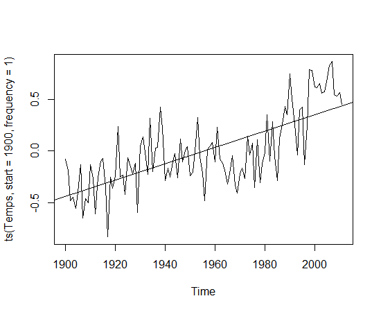
plot(ts(Temps, start =1900, frequency = 1))
abline(reg = lm(Temps~TIME))

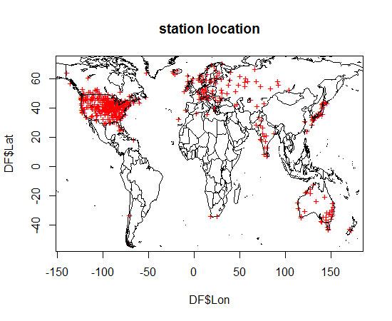
What we see should come as no surprise. The planet is getting warmer. The slope of the line is roughly  .08C/ decade.  The stations have the following geographical distribution:

The sum total of all stations is  478. The result, as we expect, is similar to the results we get if we use all stations, regardless of their length. However, we can note that the sample isn’t very representative so their could be bias due to spatial sampling.  The overweighting of the northern hemisphere is likely to cause a trend that is slightly higher than a what we would see if the sample included more SH stations.

The next step I will merely describe in words because I will probably change the code I used here when I decide upon a final approach. After calculating the global average of all these long stations I then created trends and confidence intervals for every station. For trends I used a Theil-Sen estimator which may be a bit different than most folks are used to. Its described here: http://en.wikipedia.org/wiki/Theil%E2%80%93Sen_estimator. The zyp package has a quick implementation that spits out confidence intervals as well. I’ll play around with some of Lucia’s approaches and maybe look at Tamino’s approach, but for now, this will do.

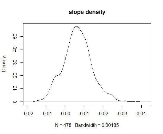
Summarizing the trends we see the following:

summary(DF$Slope) Min. 1st Qu. Median Mean 3rd Qu. Max. -0.014450 0.001390 0.006038 0.006151 0.010850 0.036920

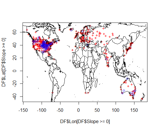
Note that the simple meanof all slopes is less than the area weighted global solution. And note that some of the slopes of individual stations are negative. These are so called cooling stations: A crude map below gives you an indication of their locations. Blue is cooling, red is warming. The warming were drawn first so they tend to get covered up.

Well there you have it. Some long stations cool.  This is fairly well known but a week doesnt pass on the internet without somebody asking about it or pointing to it as proof of “something.” Before we dive into that there is a bit more work to do.

More in the next post..