Want to share your content on R-bloggers? click here if you have a blog, or here if you don't.
This is an exciting release of futile.matrix, which in some ways the package grows up and finds its purpose. It now includes a suite of functions for generating random matrices and can be used in conjunction with RMTstat. In short, futile.matrix has two purposes:
- Investigating the properties of random matrices
- Fitting distributions and finding the upper cutoff on the noise part of the eigenvalue spectrum
This post will focus on the first purpose, that of exploring random matrices. It is meant to be an overview of functions available in the package and not a rigorous treatment of the subject matter.
Random Matrices
The package provides a number of types for describing random matrices. These types are strictly model parameters that are used to generate random matrices. Supported matrix classes include Wigner matrices, Wishart matrices, and Jacobian matrices.
Wigner Matrix
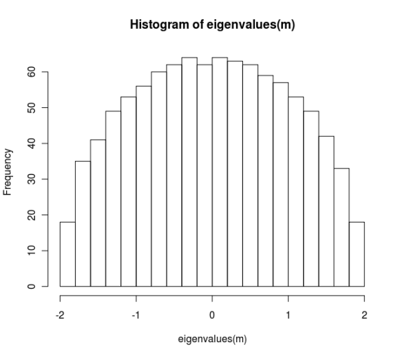
A Wigner matrix is a symmetric matrix with random Gaussian entries. To generate a matrix of this class we can create a model and then call the matrix generator. Once we create a matrix we can plot a histogram of the eigenvalues, which conforms to the Wigner semicircle law.
model <- create(WignerModel, 1000)
mat <- rmatrix(model)
hist(eigenvalues(m), breaks=20)
Additional arguments can be passed into the model to specify, for example, whether the entries are real or complex. To visually verify that the entries look correct, use the peek function.
> model <- create(WignerModel, 1000, real=FALSE)
> m <- rmatrix(model)
> peek(m)
                          [,1]                    [,2]
[1,]  0.024964162+0.000000000i  0.02515425-0.00411280i
[2,]  0.025154249+0.004112805i -0.03926107+0.00000000i
[3,] -0.001786425+0.002332125i -0.02215823-0.00532748i
[4,]  0.003182095+0.012343427i -0.05085979-0.02496951i
[5,]  0.022302859-0.006057670i -0.00372532-0.01257203i
                          [,3]                    [,4]                    [,5]
[1,] -0.001786425-0.002332125i  0.00318209-0.01234343i  0.02230286+0.00605767i
[2,] -0.022158230+0.005327478i -0.05085979+0.02496951i -0.00372532+0.01257203i
[3,] -0.041233230+0.000000000i -0.03274875-0.01665794i -0.01389319+0.00570893i
[4,] -0.032748746+0.016657935i  0.01681741+0.00000000i -0.03047206+0.00500749i
[5,] -0.013893195-0.005708930i -0.03047206-0.00500749i  0.01964392+0.00000000i
Note that when the matrix is generated, the function automatically asserts that the transpose is equal to the matrix itself via futile.paradigm.
rmatrix %must% (result == ct(result))
As expected, the histogram for this variant also conforms to the semi-circle law.
Wishart Matrix
In finance, a more useful matrix is a Wishart matrix, which is a sample covariance matrix. These matrices have an eigenvalue spectrum that is described by the Marcenko-Pastur distribution.
As an example, we’ll create a random Wishart matrix that is similar to two years of daily data on the S&P 500. We plot the actual distribution of eigenvalues alongside the theoretical distribution (generated from the RMTstat package).
model <- create(WishartModel, 500, 500)
mat <- rmatrix(model)
x <- seq(0,4, by=0.1)
par(mfrow=c(1,2))
hist(eigenvalues(m), breaks=20)
plot(x, dmp(x, svr=1), main="Theoretical distribution")
Fitting the spectrum to a theoretical curve enables you to isolate the noise part of the spectrum. Once this is established, it’s possible to clean the source correlation matrix and remove the estimation error.
Matrix Ensembles
Additional properties of random matrices can be discerned by analyzing ensembles of said matrices. We can generate the ensemble based on an existing model along with a count. Since an ensemble contains many random matrices, there is no practical way of displaying its contents. Hence, only some basic information is printed to reduce screen clutter.
</pre>
> model <- create(WishartModel, 100, 400)
> e <- create(Ensemble, 200, model)
> hist(max_eigen(e), freq=FALSE, breaks=20)
<pre>
Conclusion
This post covered the basic functions of futile.matrix and how one can analyze random matrices and their ensembles using the package. In a subsequent post, we’ll cover using the package to fit distributions and identifying the cutoff point for the noise portion of the eigenvalue spectrum.
R-bloggers.com offers daily e-mail updates about R news and tutorials about learning R and many other topics. Click here if you're looking to post or find an R/data-science job.
Want to share your content on R-bloggers? click here if you have a blog, or here if you don't.


